ROMS/TOMS Developers

Algorithms Update Web Log
Next Page »

arango - April 7, 2007 @ 0:38
IS4DVAR and Hessian Preconditioning- Comments (0)

We have been working on the new conjugate gradient algorithms for IS4DVAR for awhile. A full description of the conjugate gradient algorithm is given in Fisher and Courtier (1995), ECMWF Tech Memo 220. Many thanks to Mike Fisher for providing us his prototype code and Andy Moore for adapting it to ROMS framework.

Currently we have two conjugate gradient algorithms: cgradient.h and cgradient_lanczos.h. The cgradient.h algorithm was decribed in previous post. The new alogorithm cgradient_lanczos.h is used when the LANCZOS CPP option is activated. This routine exploits the close connection between the conjugate gradient minimization and the Lanczos algorithm:

     q(k) = g(k) / ||g(k)||

If we eliminate the descent directions (Eqs 5d and 5g) and multiply by the Hessian matrix, we get the Lanczos recurrence relationship:

     H q(k+1) = γ(k+1) q(k+2) + δ(k+1) q(k+1) + γ(k) q(k)

with

     δ(k+1) = (1 / α(k+1)) + (β(k+1) / α(k))

     γ(k) = - SQRT ( β(k+1)) / α(k) )

since the gradient and Lanczos vectors are mutually orthogonal the recurrence maybe written in matrix form as:

     H Q(k) = Q(k) T(k) + γ(k) q(k+1) e'(k)

with


             { q(1), q(2), q(3), ..., q(k) }
     Q(k) =  {  .     .     .          .   }
             {  .     .     .          .   }
             {  .     .     .          .   }

             { δ(1)  γ(1)                             }
             { γ(1)  δ(2)  γ(2)                       }
             {         .         .         .          }
     T(k) =  {          .         .         .         }
             {           .         .         .        }
             {              γ(k-2)   δ(k-1)   γ(k-1)  }
             {                       γ(k-1)   δ(k)    }

     e'(k) = { 0, ...,0, 1 }

The eigenvalues of T(k) and the vectors formed by Q(k)*T(k) are approximations to the eigenvalues and eigenvectors of the Hessian. They can be used for preconditioning.

The tangent linear model conditions and associated adjoint in terms of the Lanzos algorithm are:


     X(k) = X(0) + Q(k) Z(k)

     T(k) Z(k) = - transpose[Q(k0)] g(0)

where

     k           Inner loop iteration
     α(k)        Conjugate gradient coefficient
     β(k)        Conjugate gradient coefficient
     δ(k)        Lanczos algorithm coefficient
     γ(k)        Lanczos algorithm coefficient
     H           Hessian matrix
     Q(k)        Matrix of orthonormal Lanczos vectors
     T(k)        Symmetric, tri-diagonal matrix
     Z(k)        Eigenvectors of Q(k)*T(k)
     e'(k)       Tansposed unit vector
     g(k)        Gradient vectors (adjoint solution: GRAD(J))
     q(k)        Lanczos vectors
     <...>       Dot product
     ||...||     Euclidean norm, ||g(k)|| = SQRT( <g(k),g(k)> )

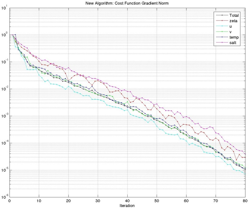
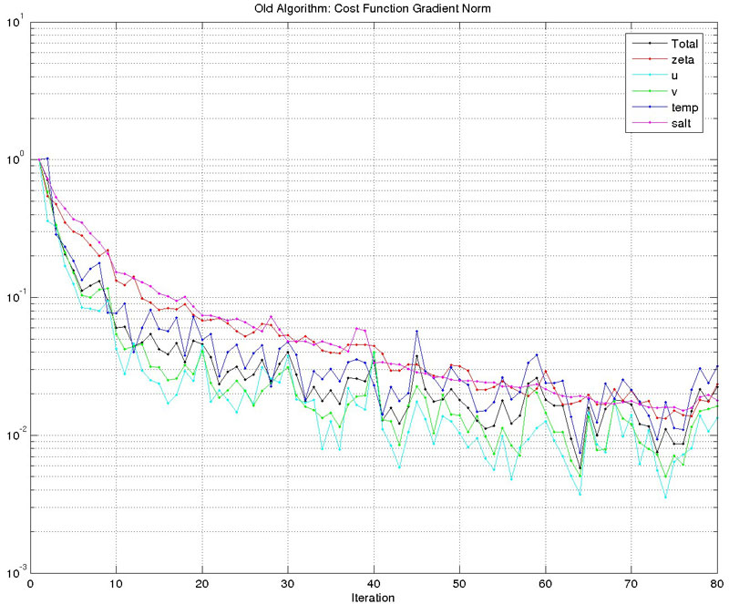
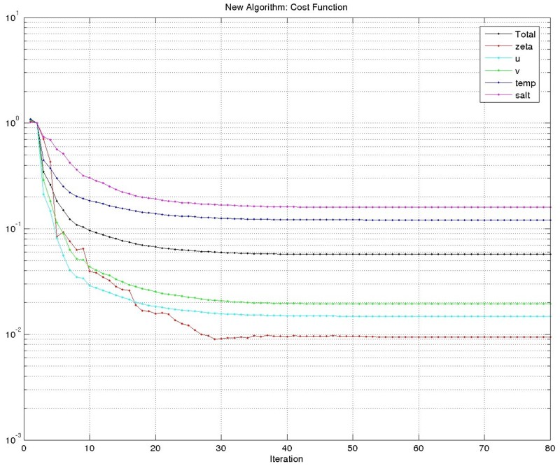
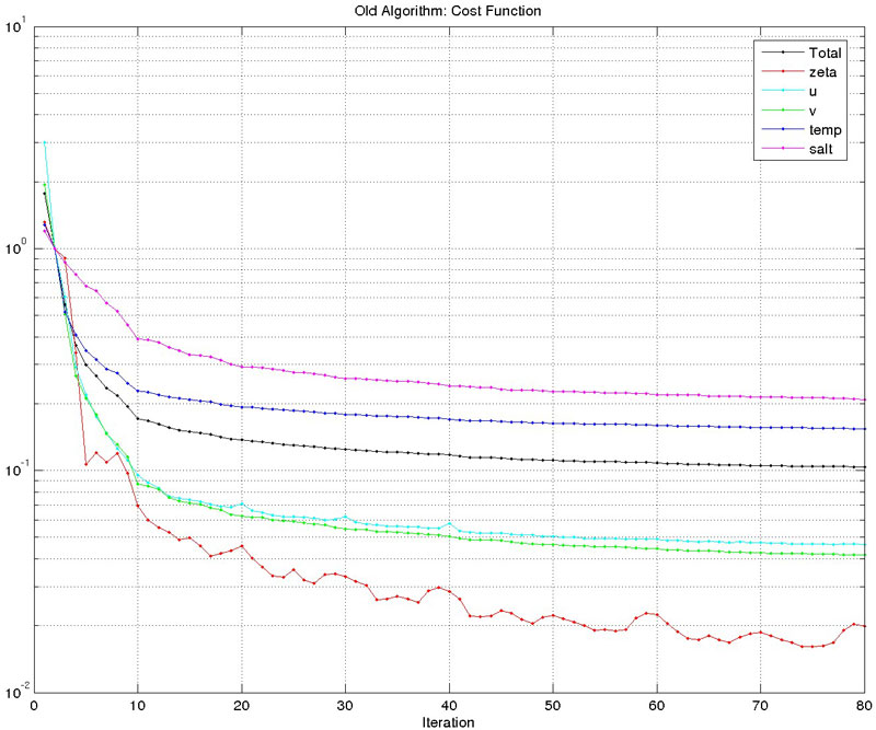
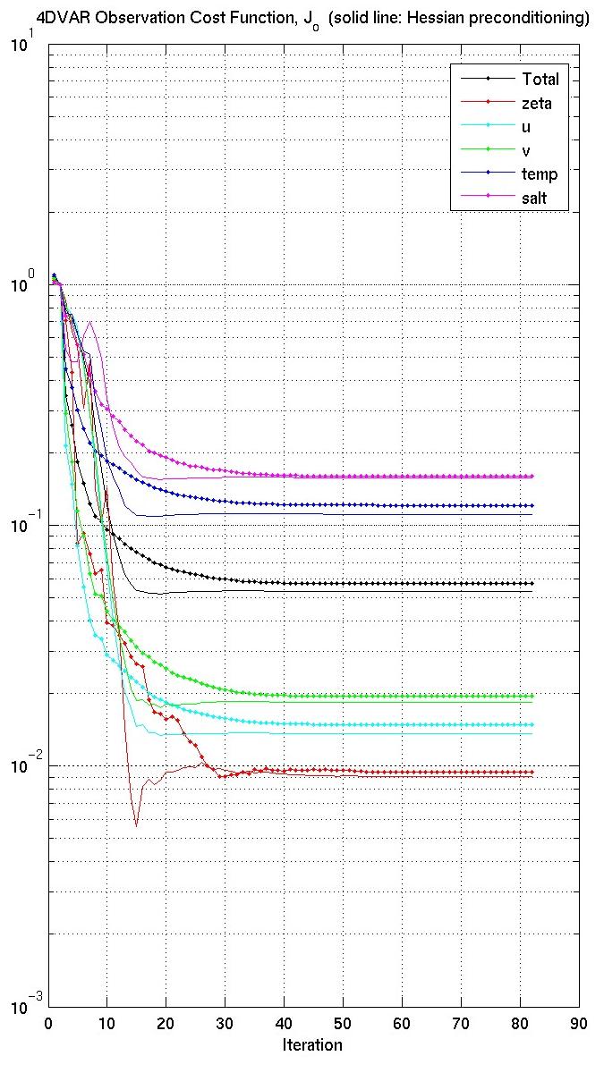
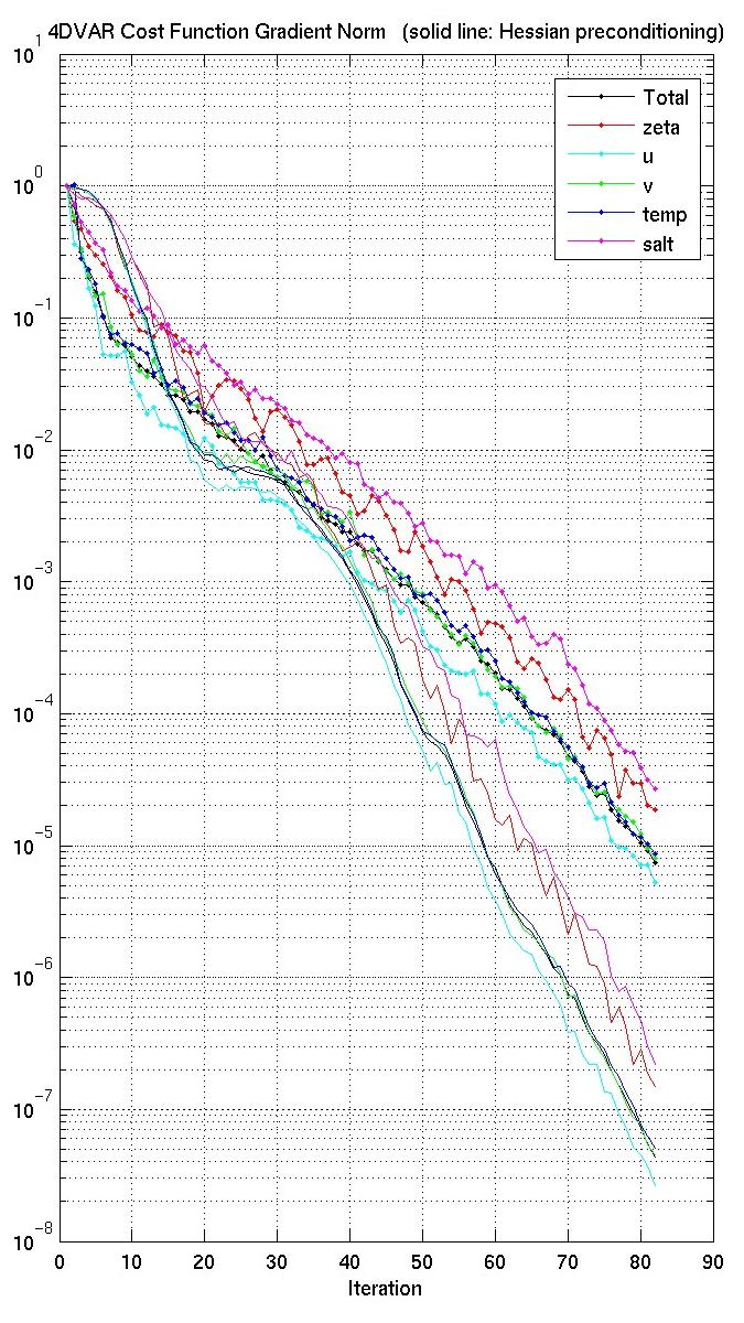
The figures below show the cost function and gradient norm for a double gyre run with (solid) and without (solid and dots) preconditioning. Notice that the preconditioned cost function has smaller values. The big improvement, however, is in the gradient norm. These results show the same behavior as that described in Mike Fisher unpublished manuscript. So we conclude that the new conjugate gradient algorithms are working very well.

Cost Function with Hessian Preconditioning

Gradient Norm with Hessian Preconditioning

Therefore, the strategy is to run both algorithms for a particular application. If the observations are in the same locations, the Hessian eigenvectors need to be computed only once and saved into HSSname NetCDF file using the LANCZOS CPP option (cgradient_lanczos.h) and logical switch LhessianEV = .TRUE.. Then, these eigenvalues and eigenvectors can be read by the cgradient.h (LANCZOS off) with logical (Lprecond = .TRUE.) to approximate the Hessian during preconditioning. We prefer the cgradient.h algorithm because we can compute the value of the cost function at each inner loop iteration. In the Lanczos algorithm (cgradient_lanczos.h) we only know the value of the cost function at the last inner loop. Notice that both algorithm (not shown) give very similar solutions.


arango - January 19, 2007 @ 17:25
New IS4DVAR Driver- Comments (0)

Added a new incremental, strong contraint 4DVAR driver which uses the conjugate gradient algorithm proposed by Mike Fisher (ECMWF). Many thanks to Mike for providing us his unpublished manuscript (Efficient Minimization of Quadratic Penalty Functions, 1997) and prototype source code. Many thanks to Andy Moore for his help in the debugging of the new algorithm.

The new driver is more efficient since only one call to the tangent linear model is needed per inner loop iteration. The old algorithm required a second call to compute the optimum conjugate gradient algorithm step size. The new algorithm can be activated with cpp option IS4DVAR and the old with IS4DVAR_OLD.

The developing of this new driver has been done in two stages:

  • Basic conjugate gradient algorithm where the new initial conditions increment and its associated gradient are adjusted to the optimum line search. In addition, the new gradient at each inner loop iteration is orthogonalized against all previous gradient using the modified Gramm-Schmidt algorithm.
  • Lanczos algorithm to compute the eigenvectors and eigenvalues used to estimate the minimization Hessian matrix for preconditioning.

Currently, only the first stage is available. The new conjugate gradient cgradient.F follows Fisher (1997) algorithm:

Given an initial increment X(0), gradient G(0), descent direction d(0)=-G(0), and trial step size τ(0) , the minimization algorithm at the k-iteration is:

  • Run tangent linear model initialized with trial step, Xhat(k), Eq 5a:

    Xhat(k) = X(k) + tau(k) * d(k)

  • Run adjoint model to compute gradient at trial point, Ghat(k), Eq 5b:

    Ghat(k) = GRAD[ f(Xhat(k)) ]

  • Compute optimum step size, α(k), Eq 5c:

    α(k) = τ(k) * <d(k),G(k)> / (<d(k),G(k)> – <d(k),Ghat(k)>)

    here <…> denotes dot product.

  • Compute new starting point (TLM increments), X(k+1), Eq 5d:

    X(k+1) = X(k) + α(k) * d(k)

  • Compute gradient at new point, G(k+1), Eq 5e:

    G(k+1) = G(k) + (alpha(k) / tau(k)) * (Ghat(k) – G(k))

  • Orthogonalize new gradient, G(k+1), against all previous gradients [G(k), …, G(0)], in reverse order, using the modified Gramm-Schmidt algorithm. Notice that we need to save all inner loop gradient solutions. Currently, all the gradients are stored in the adjoint NetCDF file(s) and not in memory.
  • Compute new descent direction, d(k+1), Eqs 5g and 5f:

    β(k+1) = <G(k+1),G(k+1)> / <G(k),G(k)>

    d(k+1) = – G(k+1) + β(k+1) * d(k)

    After the first iteration, the trial step size is:

    τ(k) = α(k-1)

The new driver is is4dvar_ocean.h and the old becomes is4dvar_ocean_old.h. The old driver is kept for comparison and will become obsolete in the future. A new generic dot product routine state_dotprod.F is introduced.

The new algorithm is still under testing but the results are promising as shown below for the double gyre test case (outer=1, inner=80 for both new and old drivers). Notice that the gradient norm in the new algorithm decreased by about five-orders of magnitude compared to only two-orders of magnitude in the old algorithm. The new algorithm is much cheaper.

Cost Function Gradient Norm, new algorithm

Cost Function Gradient Norm, old algorithm

The minimization of the cost function is also improved.

Cost Function, new algorithm

Cost Function, old algorithm

For the current updated file list .

arango - November 30, 2006 @ 1:07
Verification Option and few bugs- Comments (2)

Added a VERIFICATION option that allows to compute nonlinear model solution at observation locations. This option is independent of any of the variational data assimilation options. However, it uses the same observation interface. Like in the 4DVAR drivers, the model solution at the observation locations and the model-observation statistics are written to MODname NetCDF file. Many thanks to Brian Powell for this suggestion.

I modified and updated several routines:

  • Modified nl_ocean.h to allow computing and saving of the nonlinear model solution at the observation spatial and temporal locations. Several routines associated with data assimilation were changed slightly to accomplish this: cppdefs.h, globaldefs.h, checkdefs.F, def_mod.F, extract_obs.F, initial.F, inp_par.F, mod_fourdvar.F, mod_ncparam.F, mod_scalars.F, obs_read.F, obs_write.F, and output.F. Mostly all the changes involve adding VERIFICATION to few CPP directives.
  • Corrected a couple of adjoint bugs in ad_set_vbc.F and ini_adjust.F. These bugs only affects 2D applications and 2D optimal perturbations. Many thanks to Andy Moore for finding and correctiong these bugs.
  • Renamed routine stats_4dvar.F to a more appropriate stats_modobs.F. This implied changes in is4dvar_ocean.h, s4dvar_ocean.h, w4dpsas_ocean.h, and w4dvar_ocean.h.
  • Corrected parallel bugs in grid_coords.F and interpolate.F when computing the initial locations of stations and floats from (lon,lat) data. This bug was reported in the ROMS forum by Wen Long.
  • Corrected an array out-of-bounds in nf_fread.F in distributed-memory applications. The scratch variable wrk need to be allocated as Npts+2 since the minimum and maximum values are appended to the end of wrk in routine mp_scatter to reduce additional parallel reduction. Many thanks to John Warner for bringing this to my attention. This one was a hard one.
  • Corrected bugs in ecosim.h to fix how pigment biomass is computed. Many thanks to Bronwyn for fixing this one.
  • Corrected a typo in wrt_station.F. Many thanks to Jacopo for finding this one.
  • Corrected computation of volume-averaged kinetic energy in diag.F, ad_diag.F, rp_diag.F, and tl_diag.F as reported by Bin Zhang and Sasha in the forum.
  • Correct several parallel bugs when processing point data in set_data.F, ad_set_data.F, rp_set_data.F, and tl_set_data.F. Many thanks to Rob Hetland for finding this one.
For the current updated file list .

arango - September 25, 2006 @ 22:29
Changes to PSAS Algorithm- Comments (0)

Corrected a couple of bugs in the W4DPSAS driver:

  • Remove the writing of the nonlinear model initial conditions at the end of the inner loop in w4dpsas_ocean.h. The correction due to data assimilation is added in main3d.F to the first guess state. The nonlinear model is always started from the first guess. Otherwise, the solution dynamical range with accumulates in each outer loop. The final (optimal) nonlinear initial conditions are written after done with data assimilation.
  • Modified def_rst.F, wrt_rst.F, tl_def_his.F, and tl_wrt_his.F to write the basic state vertical mixing coefficients when any of the vertical parameterization are activated. This will allow to control instabilities due to data assimilation. Recall that the finite amplitude tangent linear model (RPM) is used as the basic state for the next outer loop iteration in the W4DVAR algorithm. Since we are not using the tangent linear of these vertical parameterizations, the nonlinear model values are a good approximation in the Picard iterations.
For the current updated file list .

arango - September 16, 2006 @ 17:10
Model-Observation Comparison Statistics- Comments (0)

Made few changes to allow model-observation comparison statistics after the 4DVAR data assimilation. Many thanks to Andy and Brian for their suggestions.

  • Modified is4dvar_ocean.h so the nonlinear model is run at the end after data assimilation, when using IS4DVAR. The nonlinear model is initialized with the estimated initial conditions from data assimilation. The nonlinear model is then interpolated at the observation locations for comparison statistics.
  • Added a new routine Utility/stats_4dvar.F to compute model-observation comparisons. The following measurements are computed for each state variable:

    1) Observations mean (obs_mean) and standard deviation (obs_std).
    2) Model mean (model_mean) and standard deviation (model_std).
    3) Model bias (model_bias).
    4) Model-Observations standard deviation error (SDE).
    5) Model-Observations cross-correlation (CC).
    6) Model-Observations mean squared error (MSE).

    All these statistical quantities are written into 4DVAR output NetCDF file (MODname) and standard output file.

  • Added stats_4dvar calls to all 4DVAR data assimilation drivers: is4dvar_ocean.h, s4dvar_ocean.h, w4dpsas_ocean.h, and w4dvar_ocean.h.
  • Fixed an out-range index bound in arrayd A2d and A3d in the exact background error normalization coefficients routine normalization.F. This is a benign bug.
  • Made changes to inp_par.F to insure that there is only one record in the restart file after the nonlinear model is run at the end of an assimilation cycle. The parameter nRST is set to ntimes. The restart file can be used as the first guess for the next assimilation file in sequential data assimilation.
For the current updated file list .