RBL4D-Var Tutorial: Difference between revisions
No edit summary (change visibility) |
No edit summary (change visibility) |
||
| Line 37: | Line 37: | ||
#Execute the configuration [[job_psas|job_psas.sh]] '''before''' running the model. It copies the required files and creates <span class="twilightBlue">psas.in</span> input script from template '''[[s4dvar.in]]'''. This has to be done '''every time''' that you run this application. We need a clean and fresh copy of the initial conditions and observation files since they are modified by ROMS during execution. | #Execute the configuration [[job_psas|job_psas.sh]] '''before''' running the model. It copies the required files and creates <span class="twilightBlue">psas.in</span> input script from template '''[[s4dvar.in]]'''. This has to be done '''every time''' that you run this application. We need a clean and fresh copy of the initial conditions and observation files since they are modified by ROMS during execution. | ||
#Run ROMS with data assimilation:<div class="box"><span class="red">mpirun -np 4 oceanM ocean_wc13.in > & log &</span></div> | #Run ROMS with data assimilation:<div class="box"><span class="red">mpirun -np 4 oceanM ocean_wc13.in > & log &</span></div> | ||
==Results== | |||
The 4D-PSAS cost function value for each inner loop iteration is shown below: | |||
[[Image:psas_cost.png|500px|thumb|left|<center>4D-PSAS Cost Function</center>]] | |||
<div style="clear: both;"></div> | |||
The total cost function '''J''' (black curve), observation cost function '''J<sub>o</sub>''' (blue curve), and background cost function '''J<sub>b</sub>''' (red curve) are plotted on a log<sub>10</sub> scale. The value of the nonlinear cost function '''J<sub>NL</sub>''' at the end of the inner loops is also shown (red X). The horizontal, dashed line shows the theoretical '''J<sub>min</sub>'''. | |||
---- | |||
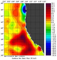
The 4D-PSAS initial conditions increments for free-surface (m), surface wind stress components (Pa), and surface net heat flux (W/m<sup>2</sup>) are shown below: | |||
{| | |||
|- | |||
|[[Image:psas_increments_fs.png|thumb|200px|<center>Free-surface</center>]] | |||
|[[Image:psas_increments_uwind.png|thumb|200px|<center>τ<sub>x</sub></center>]] | |||
|[[Image:psas_increments_vwind.png|thumb|200px|<center>τ<sub>y</sub></center>]] | |||
|[[Image:psas_increments_heat.png|thumb|200px|<center>Net Heat Flux</center>]] | |||
|} | |||
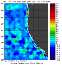
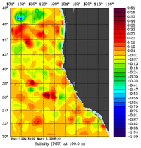
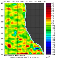
The 4D-PSAS initial conditions increments at 100m for temperature (°C), salinity, and momentum components (m/s) are shown below: | |||
{| | |||
|- | |||
|[[Image:psas_increments_T.png|thumb|200px|<center>Temperature</center>]] | |||
|[[Image:psas_increments_S.png|thumb|200px|<center>Salinity</center>]] | |||
|[[Image:psas_increments_u.png|thumb|200px|<center>U-Momentum</center>]] | |||
|[[Image:psas_increments_v.png|thumb|200px|<center>V-Momentum</center>]] | |||
|} | |||
A cross-section along 37°N for the 4D-PSAS initial conditions increments is shown below. | |||
{| | |||
|- | |||
|[[Image:psas_increments_sec_T.png|thumb|200px|<center>Temperature</center>]] | |||
|[[Image:psas_increments_sec_S.png|thumb|200px|<center>Salinity</center>]] | |||
|[[Image:psas_increments_sec_u.png|thumb|200px|<center>U-Momentum</center>]] | |||
|[[Image:psas_increments_sec_v.png|thumb|200px|<center>V-Momentum</center>]] | |||
|} | |||
---- | |||
4D-PSAS posterior analysis error covariance EOF eigenvalues and randomization trace estimates. | |||
[[Image:psas_eof_eigenvalues.png|500px|thumb|left|<center>4D-PSAS EOF Eigenvalues</center>]] | |||
<div style="clear: both;"></div> | |||
---- | |||
The 4D-PSAS posterior analysis error covariance (EOF 1) for free-surface (m), surface wind stress components (Pa), and surface net heat flux (W/m<sup>2</sup>) are shown below: | |||
{| | |||
|- | |||
|[[Image:psas_posterior_EOF_fs.png|thumb|200px|<center>Free-surface</center>]] | |||
|[[Image:psas_posterior_EOF_uwind.png|thumb|200px|<center>τ<sub>x</sub></center>]] | |||
|[[Image:psas_posterior_EOF_vwind.png|thumb|200px|<center>τ<sub>y</sub></center>]] | |||
|[[Image:psas_posterior_EOF_heat.png|thumb|200px|<center>Net Heat Flux</center>]] | |||
|} | |||
The 4D-PSAS posterior analysis error covariance (EOF 1) at 100m for temperature (°C), salinity, and momentum components (m/s) are shown below: | |||
{| | |||
|- | |||
|[[Image:psas_posterior_EOF_T.png|thumb|200px|<center>Temperature</center>]] | |||
|[[Image:psas_posterior_EOF_S.png|thumb|200px|<center>Salinity</center>]] | |||
|[[Image:psas_posterior_EOF_u.png|thumb|200px|<center>U-Momentum</center>]] | |||
|[[Image:psas_posterior_EOF_v.png|thumb|200px|<center>V-Momentum</center>]] | |||
|} | |||
A cross-section along 37°N for the 4D-PSAS posterior analysis error covariance (EOF 1) is shown below. | |||
{| | |||
|- | |||
|[[Image:psas_posterior_EOF_sec_T.png|thumb|200px|<center>Temperature</center>]] | |||
|[[Image:psas_posterior_EOF_sec_S.png|thumb|200px|<center>Salinity</center>]] | |||
|[[Image:psas_posterior_EOF_sec_u.png|thumb|200px|<center>U-Momentum</center>]] | |||
|[[Image:psas_posterior_EOF_sec_v.png|thumb|200px|<center>V-Momentum</center>]] | |||
|} | |||
==References== | ==References== | ||
The technical description of the algorithms and application used in this tutorial are described in Moore ''et al.'' ([[Bibliography#MooreAM_2010a|2010a]], [[Bibliography#MooreAM_2010b|b]], [[Bibliography#MooreAM_2010c|c]]). | The technical description of the algorithms and application used in this tutorial are described in Moore ''et al.'' ([[Bibliography#MooreAM_2010a|2010a]], [[Bibliography#MooreAM_2010b|b]], [[Bibliography#MooreAM_2010c|c]]). | ||
Revision as of 22:46, 30 June 2010
The various files in the PSAS folder are needed to run the strong/weak constraint, dual form of 4-Dimensional Variational (4D-Var) data assimilation based on the Physical-space Statistical Analysis System (PSAS) algorithm in the California Current System, 1/3° resolution, application (WC13).
![]() This page is under construction
This page is under construction![]()
Important CPP Options
POSTERIOR_EOFS Estimate posterior analysis error
POSTERIOR_ERROR_I Estimate initial posterior analysis error
WC13 Application CPP option
Input NetCDF Files
Nonlinear Initial File: wc13_ini.nc
Forcing File 01: ../Data/coamps_wc13_lwrad_down.nc
Forcing File 02: ../Data/coamps_wc13_Pair.nc
Forcing File 03: ../Data/coamps_wc13_Qair.nc
Forcing File 04: ../Data/coamps_wc13_rain.nc
Forcing File 05: ../Data/coamps_wc13_swrad.nc
Forcing File 06: ../Data/coamps_wc13_Tair.nc
Forcing File 07: ../Data/coamps_wc13_wind.nc
Boundary File: ../Data/wc13_ecco_bry.nc
Initial Conditions STD File: ../Data/wc13_std_i.nc
Model STD File: ../Data/wc13_std_m.nc
Boundary Conditions STD File: ../Data/wc13_std_b.nc
Surface Forcing STD File: ../Data/wc13_std_f.nc
Initial Conditions Norm File: ../Data/wc13_nrm_i.nc
Model Norm File: ../Data/wc13_nrm_m.nc
Boundary Conditions Norm File: ../Data/wc13_nrm_b.nc
Surface Forcing Norm File: ../Data/wc13_nrm_f.nc
Observations File: wc13_obs.nc
Various Scripts and Include Files
build.sh csh Unix script to compile application
job_psas.sh job configuration script
ocean_wc13.in ROMS standard input script for WC13
s4dvar.in 4D-Var standard input script template
wc13.h WC13 header with CPP options
Instructions
To run this application you need to take the following steps:
- We need to run the model application for a period that is long enough to compute meaningful circulation statistics, like mean and standard deviations for all prognostic state variables (zeta, u, v, T, and S). The standard deviations are written to NetCDF files and are read by the 4D-Var algorithm to convert modeled error correlations to error covariances. The error covariance matrix, D, is very large and not well known. It is modeled as the solution of a diffusion equation as in Weaver and Courtier (2001).In this application, we need standard deviations for initial conditions, surface forcing (ADJUST_WSTRESS and ADJUST_STFLUX), and open boundary conditions (ADJUST_BOUNDARY). The standard deviations for the initial and open boundary conditions are in terms of the unbalanced error covariance (K Du KT) since the balanced operator is activated (BALANCE_OPERATOR and ZETA_ELLIPTIC).The balance operator imposes a multivariate constraint on the error covariance such that the unobserved variable information is extracted from observed data by establishing balance relationships (i.e., T-S empirical formulas, hydrostactic balance, and geostrophic balance) with other state variables (Weaver et al., 2005).These standard deviations have already been created for you:../Data/wc13_std_i.nc initial conditions
../Data/wc13_std_m.nc model error (if weak constraint)
../Data/wc13_std_b.nc open boundary conditions
../Data/wc13_std_f.nc surface forcing (wind stress and net heat flux) - Since we are modeling the error covariance matrix, D, we need to compute the normalization coefficients to ensure that the diagonal elements of the associated correlation matrix C are equal to unity. There are two methods to compute normalization coefficients: exact and randomization (an approximation).The exact method is very expensive on large grids. The normalization coefficients are computed by perturbing each model grid cell with a delta function scaled by the area (2D state variables) or volume (3D state variables), and then by convolving with the squared-root adjoint and tangent linear diffusion operators.The approximate method is cheaper: the normalization coefficients are computed using the randomization approach of Fisher and Courtier (1995). The coefficients are initialized with random numbers having a uniform distribution (drawn from a normal distribution with zero mean and unit variance). Then, they are scaled by the inverse squared-root of the cell area (2D state variable) or volume (3D state variable) and convolved with the squared-root adjoint and tangent diffusion operators over a specified number of iterations, Nrandom.Check following parameters in the 4D-Var input script s4dvar.in (see input script for details):Nmethod == 0 ! normalization methodThese normalization coefficients have already been computed for you (../Normalization) using the exact method since this application has a small grid (54x53x30):
Nrandom == 5000 ! randomization iterations
LdefNRM == F F F F ! Create a new normalization files
LwrtNRM == F F F F ! Compute and write normalization
CnormI(isFsur) = T ! 2D variable at RHO-points
CnormI(isUbar) = T ! 2D variable at U-points
CnormI(isVbar) = T ! 2D variable at V-points
CnormI(isUvel) = T ! 3D variable at U-points
CnormI(isVvel) = T ! 3D variable at V-points
CnormI(isTvar) = T T ! NT tracers
CnormB(isFsur) = T ! 2D variable at RHO-points
CnormB(isUbar) = T ! 2D variable at U-points
CnormB(isVbar) = T ! 2D variable at V-points
CnormB(isUvel) = T ! 3D variable at U-points
CnormB(isVvel) = T ! 3D variable at V-points
CnormB(isTvar) = T T ! NT tracers
CnormF(isUstr) = T ! surface U-momentum stress
CnormF(isVstr) = T ! surface V-momentum stress
CnormF(isTsur) = T T ! NT surface tracers flux../Data/wc13_nrm_i.nc initial conditionsNotice that the switches LdefNRM and LwrtNRM are all false (F) since we already computed these coefficients.
../Data/wc13_nrm_m.nc model error (if weak constraint)
../Data/wc13_nrm_b.nc open boundary conditions
../Data/wc13_nrm_f.nc surface forcing (wind stress and
net heat flux)The normalization coefficients need to be computed only once for a particular application provided that the grid, land/sea masking (if any), and decorrelation scales (HdecayI, VdecayI, HdecayB, VdecayV, and HdecayF) remain the same. Notice that large spatial changes in the normalization coefficient structure are observed near the open boundaries and land/sea masking regions. - Customize your preferred build script and provide the appropriate values for:
- Root directory, MY_ROOT_DIR
- ROMS source code, MY_ROMS_SRC
- Fortran compiler, FORT
- MPI flags, USE_MPI and USE_MPIF90
- Path of MPI, NetCDF, and ARPACK libraries according to the compiler. Notice that you need to provide the correct places of these libraries for your computer. If you want to ignore this section, comment out the assignment for the variable USE_MY_LIBS.
- Notice that the most important CPP options for this application are specified in the build script instead of wc13.h:setenv MY_CPP_FLAGS "-DW4DPSAS"This is to allow flexibility with different CPP options.
setenv MY_CPP_FLAGS "${MY_CPP_FLAGS} -DPOSTERIOR_EOFS"
setenv MY_CPP_FLAGS "${MY_CPP_FLAGS} -DPOSTERIOR_ERROR_I"For this to work, however, any #undef directives MUST be avoided in the header file wc13.h since it has precedence during C-preprocessing. - You MUST use the build script to compile.
- Customize the ROMS input script ocean_wc13.in and specify the appropriate values for the distributed-memory partition. It is set by default to:Notice that the adjoint-based algorithms can only be run in parallel using MPI. This is because of the way that the adjoint model is constructed.
- Customize the configuration script job_psas.sh and provide the appropriate place for the substitute Perl script:set SUBSTITUTE=${ROMS_ROOT}/ROMS/Bin/substituteThis script is distributed with ROMS and it is found in the ROMS/Bin sub-directory. Alternatively, you can define ROMS_ROOT environmental variable in your .cshrc login script. For example, I have:setenv ROMS_ROOT /home/arango/ocean/toms/repository/trunk
- Execute the configuration job_psas.sh before running the model. It copies the required files and creates psas.in input script from template s4dvar.in. This has to be done every time that you run this application. We need a clean and fresh copy of the initial conditions and observation files since they are modified by ROMS during execution.
- Run ROMS with data assimilation:mpirun -np 4 oceanM ocean_wc13.in > & log &
Results
The 4D-PSAS cost function value for each inner loop iteration is shown below:
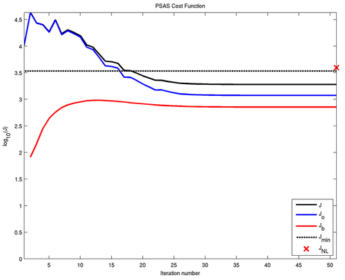
The total cost function J (black curve), observation cost function Jo (blue curve), and background cost function Jb (red curve) are plotted on a log10 scale. The value of the nonlinear cost function JNL at the end of the inner loops is also shown (red X). The horizontal, dashed line shows the theoretical Jmin.
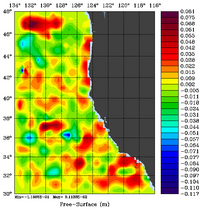
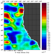
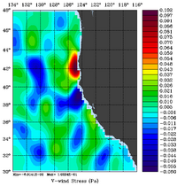
The 4D-PSAS initial conditions increments for free-surface (m), surface wind stress components (Pa), and surface net heat flux (W/m2) are shown below:
 |
 |
 |
 |
The 4D-PSAS initial conditions increments at 100m for temperature (°C), salinity, and momentum components (m/s) are shown below:
 |
 |
 |
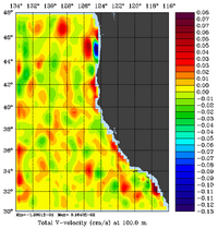 |
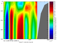
A cross-section along 37°N for the 4D-PSAS initial conditions increments is shown below.
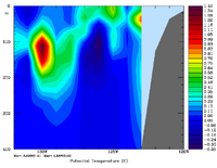 |
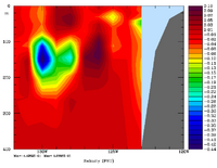 |
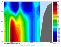 |
 |
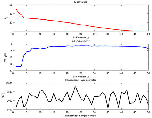
4D-PSAS posterior analysis error covariance EOF eigenvalues and randomization trace estimates.
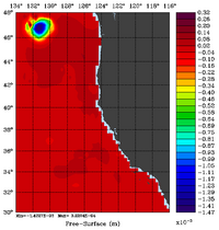
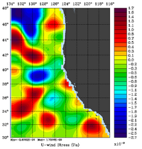
The 4D-PSAS posterior analysis error covariance (EOF 1) for free-surface (m), surface wind stress components (Pa), and surface net heat flux (W/m2) are shown below:
 |
 |
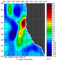 |
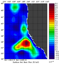 |
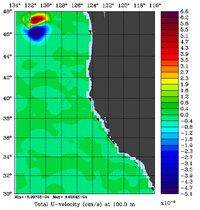
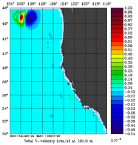
The 4D-PSAS posterior analysis error covariance (EOF 1) at 100m for temperature (°C), salinity, and momentum components (m/s) are shown below:
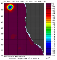 |
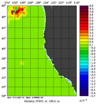 |
 |
 |
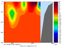
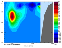
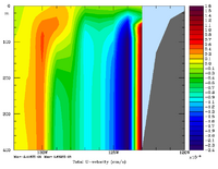
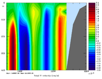
A cross-section along 37°N for the 4D-PSAS posterior analysis error covariance (EOF 1) is shown below.
 |
 |
 |
 |
References
The technical description of the algorithms and application used in this tutorial are described in Moore et al. (2010a, b, c).