RBL4D-Var Forecast Observation Impact Tutorial: Difference between revisions
No edit summary (change visibility) |
|||
| (3 intermediate revisions by 2 users not shown) | |||
| Line 17: | Line 17: | ||
#The 4-day analysis cycle of Exercise 3 is used which spans the 4-day period midnight on 3 Jan 2004 to midnight on 7 Jan 2004. The forecast interval spans the 7-day period midnight on 7 Jan 2004 to midnight on 14 Jan 2004. We will use equation (2) as a measure of the forecast error and choose '''C''' so that '''e''' is the forecast error in the 37ºN transport averaged over forecast day 7 as measured against a verifying analysis. This is indicated as the '''verifying interval''' in Fig. 1. The verifying analysis x_a was computed by running a second 4D-Var analysis cycle for the 7-day window 7-14 Jan 2004. This has been precomputed for you in these exercises. | #The 4-day analysis cycle of Exercise 3 is used which spans the 4-day period midnight on 3 Jan 2004 to midnight on 7 Jan 2004. The forecast interval spans the 7-day period midnight on 7 Jan 2004 to midnight on 14 Jan 2004. We will use equation (2) as a measure of the forecast error and choose '''C''' so that '''e''' is the forecast error in the 37ºN transport averaged over forecast day 7 as measured against a verifying analysis. This is indicated as the '''verifying interval''' in Fig. 1. The verifying analysis x_a was computed by running a second 4D-Var analysis cycle for the 7-day window 7-14 Jan 2004. This has been precomputed for you in these exercises. | ||
#We will use equation (3) as a measure forecast error. For this exercise, '''e''' is chosen to be the mean squared error in SST during forecast day 7 over the target area. | #We will use equation (3) as a measure forecast error but with metric on the observations. For this exercise, '''e''' is chosen to be the mean squared error in SST during forecast day 7 over the target area. | ||
<br \> | <br \> | ||
| Line 49: | Line 49: | ||
<div class="box"> [[Options#W4DPSAS_FCT_SENSITIVITY|W4DPSAS_FCT_SENSITIVITY]] 4D-PSAS observation sensitivity driver<br /> [[Options#ANA_SPONGE|ANA_SPONGE]] Analytical enhanced viscosity/diffusion sponge<br /> [[Options#AD_IMPULSE|AD_IMPULSE]] Force ADM with intermittent impulses<br /> [[Options#OBS_IMPACT|OBS_IMPACT]] Compute observation impact<br /> [[Options#RPCG|RPCG]] Restricted B-preconditioned Lanczos minimization<br /> [[Options#WC13|WC13]] Application CPP option</div> | <div class="box"> [[Options#W4DPSAS_FCT_SENSITIVITY|W4DPSAS_FCT_SENSITIVITY]] 4D-PSAS observation sensitivity driver<br /> [[Options#ANA_SPONGE|ANA_SPONGE]] Analytical enhanced viscosity/diffusion sponge<br /> [[Options#AD_IMPULSE|AD_IMPULSE]] Force ADM with intermittent impulses<br /> [[Options#OBS_IMPACT|OBS_IMPACT]] Compute observation impact<br /> [[Options#RPCG|RPCG]] Restricted B-preconditioned Lanczos minimization<br /> [[Options#WC13|WC13]] Application CPP option</div> | ||
For Step | For Step 8 (<span class="twilightBlue">WC13/PSAS_forecast_impact</span>) Case 2 to run ROMS 4D-PSAS Forecast Observation Impacts: | ||
<div class="box"> [[Options#W4DPSAS_FCT_SENSITIVITY|W4DPSAS_FCT_SENSITIVITY]] 4D-PSAS observation sensitivity driver<br /> [[Options#ANA_SPONGE|ANA_SPONGE]] Analytical enhanced viscosity/diffusion sponge<br /> [[Options#AD_IMPULSE|AD_IMPULSE]] Force ADM with intermittent impulses<br /> [[Options#OBS_IMPACT|OBS_IMPACT]] Compute observation impact<br /> [[Options#OBS_SPACE|OBS_SPACE]] Compute the forecast error metrics in observation space<br /> [[Options#RPCG|RPCG]] Restricted B-preconditioned Lanczos minimization<br /> [[Options#WC13|WC13]] Application CPP option</div> | <div class="box"> [[Options#W4DPSAS_FCT_SENSITIVITY|W4DPSAS_FCT_SENSITIVITY]] 4D-PSAS observation sensitivity driver<br /> [[Options#ANA_SPONGE|ANA_SPONGE]] Analytical enhanced viscosity/diffusion sponge<br /> [[Options#AD_IMPULSE|AD_IMPULSE]] Force ADM with intermittent impulses<br /> [[Options#OBS_IMPACT|OBS_IMPACT]] Compute observation impact<br /> [[Options#OBS_SPACE|OBS_SPACE]] Compute the forecast error metrics in observation space<br /> [[Options#RPCG|RPCG]] Restricted B-preconditioned Lanczos minimization<br /> [[Options#WC13|WC13]] Application CPP option</div> | ||
| Line 67: | Line 67: | ||
<div class="box"> <span class="twilightBlue">Readme</span> instructions<br /> [[build_Script|build_roms.bash]] bash shell script to compile application<br /> [[build_Script|build_roms.sh]] csh Unix script to compile application<br /> [[create_ini_fcstb.m|create_ini_fcstb.m]] Matlab script to create ROMS initial conditions<br /> [[job_fcstb.sh|job_fcstb.sh]] job configuration script<br /> [[roms.in|roms_wc13.in]] ROMS standard input script for WC13<br /> [[s4dvar.in]] 4D-Var standard input script template<br /> <span class="twilightBlue">wc13.h</span> WC13 header with CPP options</div> | <div class="box"> <span class="twilightBlue">Readme</span> instructions<br /> [[build_Script|build_roms.bash]] bash shell script to compile application<br /> [[build_Script|build_roms.sh]] csh Unix script to compile application<br /> [[create_ini_fcstb.m|create_ini_fcstb.m]] Matlab script to create ROMS initial conditions<br /> [[job_fcstb.sh|job_fcstb.sh]] job configuration script<br /> [[roms.in|roms_wc13.in]] ROMS standard input script for WC13<br /> [[s4dvar.in]] 4D-Var standard input script template<br /> <span class="twilightBlue">wc13.h</span> WC13 header with CPP options</div> | ||
For | For steps 5 and 8, the following files will be found in <span class="twilightBlue">WC13/PSAS_forecast_impact</span> directory after downloading from ROMS test cases SVN repository: | ||
<div class="box"> <span class="twilightBlue">Readme</span> instructions<br /> [[build_Script|build_roms.bash]] bash shell script to compile application<br /> [[build_Script|build_roms.sh]] csh Unix script to compile application<br /> [[job_psas_fct_impact.sh|job_psas_fct_impact.sh]] job configuration script<br /> [[roms.in|roms_wc13.in]] ROMS standard input script for WC13<br /> [[s4dvar.in]] 4D-Var standard input script template<br /> <span class="twilightBlue">wc13.h</span> WC13 header with CPP options</div> | <div class="box"> <span class="twilightBlue">Readme</span> instructions<br /> [[build_Script|build_roms.bash]] bash shell script to compile application<br /> [[build_Script|build_roms.sh]] csh Unix script to compile application<br /> [[job_psas_fct_impact.sh|job_psas_fct_impact.sh]] job configuration script<br /> [[roms.in|roms_wc13.in]] ROMS standard input script for WC13<br /> [[s4dvar.in]] 4D-Var standard input script template<br /> <span class="twilightBlue">wc13.h</span> WC13 header with CPP options</div> | ||
| Line 150: | Line 150: | ||
##Execute the configuration [[job_psas_fct_impact_obs_space.sh]] '''before''' running the model. It copies the required files and creates <span class="twilightBlue">psas.in</span> input script from template '''[[s4dvar.in]]'''. This has to be done '''every time''' that you run this application. We need a clean and fresh copy of the initial conditions and observation files since they are modified by ROMS during execution. | ##Execute the configuration [[job_psas_fct_impact_obs_space.sh]] '''before''' running the model. It copies the required files and creates <span class="twilightBlue">psas.in</span> input script from template '''[[s4dvar.in]]'''. This has to be done '''every time''' that you run this application. We need a clean and fresh copy of the initial conditions and observation files since they are modified by ROMS during execution. | ||
##Run ROMS with data assimilation:<div class="box"><span class="red">mpirun -np 8 romsM roms_wc13.in > & log &</span></div> | ##Run ROMS with data assimilation:<div class="box"><span class="red">mpirun -np 8 romsM roms_wc13.in > & log &</span></div> | ||
##We recommend creating a new subdirectory <span class="twilightBlue">Case2</span>, and saving the solution in it for analysis and plotting to avoid overwriting solutions when playing with | ##We recommend creating a new subdirectory <span class="twilightBlue">Case2</span>, and saving the solution in it for analysis and plotting to avoid overwriting solutions when playing with different CPP options. For example<div class="box">mkdir Case2<br />mv Build_roms psas.in *.nc log Case2<br />cp -p romsM roms_wc13.in Case2</div>where log is the ROMS standard output specified in the previous step. | ||
#To plot the output from step 8, go to the subdirectory <span class="twilightBlue">WC13/plotting</span> and run the Matlab script <span class="twilightBlue">plot_psas_forecast_impact_obs_space.m</span> | #To plot the output from step 8, go to the subdirectory <span class="twilightBlue">WC13/plotting</span> and run the Matlab script <span class="twilightBlue">plot_psas_forecast_impact_obs_space.m</span> | ||
| Line 158: | Line 158: | ||
{|align="center" | {|align="center" | ||
|- | |- | ||
|[[Image:psas_forecast_impact_case1_2019.png|500px|thumb|center|<center>'''Case 1:''' 7-day Forecast 37°N transport Errors</center>]] | |[[Image:psas_forecast_impact_case1_2019.png|500px|thumb|center|<center>'''Case 1:''' 7-day Forecast 37°N transport Errors<br />''prior'' saved daily</center>]] | ||
|[[Image:psas_forecast_impact_case2_2019.png|500px|thumb|center|<center>'''Case 2:''' 7-day Forecast SST Errors</center>]] | |[[Image:psas_forecast_impact_case2_2019.png|500px|thumb|center|<center>'''Case 2:''' 7-day Forecast SST Errors<br />''prior'' saved daily</center>]] | ||
|- | |||
|[[Image:psas_forecast_impact_case1_2hour_2019.png|500px|thumb|center|<center>'''Case 1:''' 7-day Forecast 37°N transport Errors<br />''prior'' saved every 2 hours</center>]] | |||
|[[Image:psas_forecast_impact_case2_2hour_2019.png|500px|thumb|center|<center>'''Case 2:''' 7-day Forecast SST Errors<br />''prior'' saved every 2 hours</center>]] | |||
|} | |} | ||
Revision as of 15:44, 30 August 2019
Introduction
A schematic representation of a typical analysis-forecast cycle using ROMS is shown in the diagram below. During the analysis cycle, a background solution (represented by the blue line) is corrected using observations that are available during the analysis window. The analysis state estimate at the end of the analysis window is then used as the initial condition for a forecast. The red curve represents the forecast generated during the forecast cycle from the 4D-Var analysis. The skill of the forecast on any day can then be assessed by comparing it to a new analysis that verifies on the same forecast day, or by comparing the forecast with new observations that have not yet been assimilated into the model.
To quantify the impact of the observations on the forecast skill it is necessary to run a second forecast which is initialized from the background solution at the end of the analysis cycle. This is represented by the green curve in Fig. 1. The difference in forecast skill between the red forecast and the green forecast is then due to the observations that were assimilated into the model during the analysis cycle.
In this tutorial, the methodology will be described by two metrics in Case 1 and Case 2:
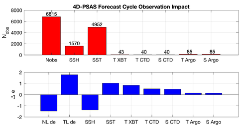
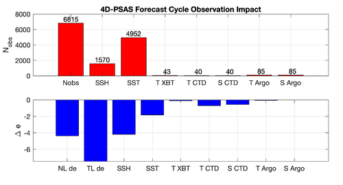
- The 4-day analysis cycle of Exercise 3 is used which spans the 4-day period midnight on 3 Jan 2004 to midnight on 7 Jan 2004. The forecast interval spans the 7-day period midnight on 7 Jan 2004 to midnight on 14 Jan 2004. We will use equation (2) as a measure of the forecast error and choose C so that e is the forecast error in the 37ºN transport averaged over forecast day 7 as measured against a verifying analysis. This is indicated as the verifying interval in Fig. 1. The verifying analysis x_a was computed by running a second 4D-Var analysis cycle for the 7-day window 7-14 Jan 2004. This has been precomputed for you in these exercises.
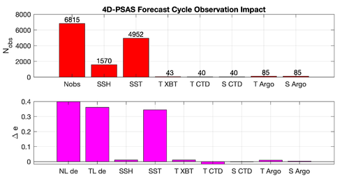
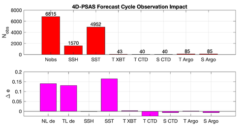
- We will use equation (3) as a measure forecast error but with metric on the observations. For this exercise, e is chosen to be the mean squared error in SST during forecast day 7 over the target area.

Model Set-up
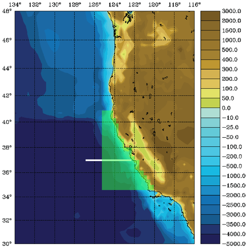
The WC13 model domain is shown in Fig. 1 and has open boundaries along the northern, western, and southern edges of the model domain.
In the tutorial, you will perform a 4D-Var data assimilation cycle that spans the period 3-6 January, 2004. The 4D-Var control vector δz is comprised of increments to the initial conditions, δx(t0), surface forcing, δf(t), and open boundary conditions, δb(t). The prior initial conditions, xb(t0), are taken from the sequence of 4D-Var experiments described by Moore et al. (2011b) in which data were assimilated every 7 days during the period July 2002- December 2004. The prior surface forcing, fb(t), takes the form of surface wind stress, heat flux, and a freshwater flux computed using the ROMS bulk flux formulation, and using near surface air data from COAMPS (Doyle et al., 2009). Clamped open boundary conditions are imposed on (u,v) and tracers, and the prior boundary conditions, bb(t), are taken from the global ECCO product (Wunsch and Heimbach, 2007). The free-surface height and vertically integrated velocity components are subject to the usual Chapman and Flather radiation conditions at the open boundaries. The prior surface forcing and open boundary conditions are provided daily and linearly interpolated in time. Similarly, the increments δf(t) and δb(t) are also computed daily and linearly interpolated in time.
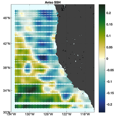
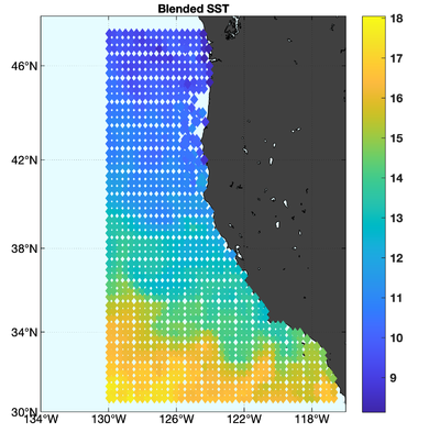
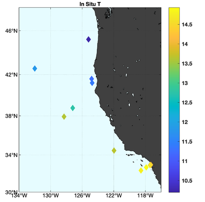
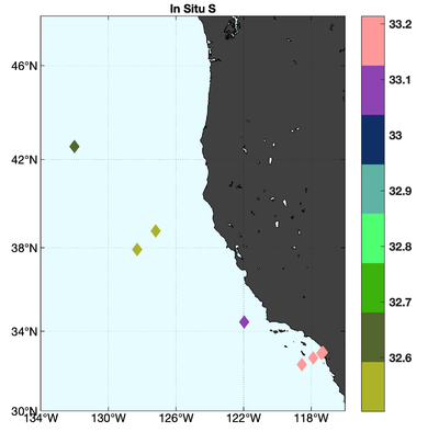
The observations assimilated into the model are satellite SST, satellite SSH in the form of a gridded product from Aviso, and hydrographic observations of temperature and salinity collected from Argo floats and during the GLOBEC/LTOP and CalCOFI cruises off the coast of Oregon and southern California, respectively. The observation locations are illustrated in Fig. 2.
 |
 |
 |
 |
Running 4D-PSAS Observation Impact
To run this exercise, go first to the directory WC13/PSAS_forecast_impact. Instructions for compiling and running the model are provided below or can be found in the Readme file. The recommended configuration for this exercise is one outer-loop and 50 inner-loops, and roms_wc13.in is configured for this default case. The number of inner-loops is controlled by the parameter Ninner in roms_wc13.in.
Important CPP Options
The following C-preprocessing options are activated in the build script:
For the intermediate Step 1 (WC13/PSAS_forecast_impact/FCSTAT) that creates the surface forcing to be use by the trajectory initialized by the 4D-PSAS analysis (WC13/PSAS_forecast_impact/FCSTA) and trajectory initialized with the background circulation (WC13/PSAS_forecast_impact/FCSTB) at the end of the 4D-PSAS cycle:
ANA_SPONGE Analytical enhanced viscosity/diffusion sponge
BULK_FLUXES Surface bulk fluxes parameterization
FORWARD_WRITE Write out Forward solution for Tangent/Adjoint
VERIFICATION Process model solution at observation locations
WC13 Application CPP option
For the intermediate Step 2 (WC13/PSAS_forecast_impact/FCSTA) to run ROMS in forecast mode initialized with the surface forcing from Step 1 (WC13/PSAS_forecast_impact/FCSTAT):
ANA_SPONGE Analytical enhanced viscosity/diffusion sponge
FORWARD_WRITE Write out Forward solution for Tangent/Adjoint
VERIFICATION Process model solution at observation locations
WC13 Application CPP option
For the intermediate Step 3 (WC13/PSAS_forecast_impact/FCSTB) to run ROMS in forecast mode initialized with the surface forcing from Step 1 (WC13/PSAS_forecast_impact/FCSTAT):
ANA_SPONGE Analytical enhanced viscosity/diffusion sponge
FORWARD_WRITE Write out Forward solution for Tangent/Adjoint
VERIFICATION Process model solution at observation locations
WC13 Application CPP option
For Step 5 (WC13/PSAS_forecast_impact) Case 1 to run ROMS 4D-PSAS Forecast Observation Impacts:
ANA_SPONGE Analytical enhanced viscosity/diffusion sponge
AD_IMPULSE Force ADM with intermittent impulses
OBS_IMPACT Compute observation impact
RPCG Restricted B-preconditioned Lanczos minimization
WC13 Application CPP option
For Step 8 (WC13/PSAS_forecast_impact) Case 2 to run ROMS 4D-PSAS Forecast Observation Impacts:
ANA_SPONGE Analytical enhanced viscosity/diffusion sponge
AD_IMPULSE Force ADM with intermittent impulses
OBS_IMPACT Compute observation impact
OBS_SPACE Compute the forecast error metrics in observation space
RPCG Restricted B-preconditioned Lanczos minimization
WC13 Application CPP option
Input NetCDF Files
WC13 requires the following input NetCDF files:
Nonlinear Initial File: wc13_ini.nc
Forcing File 01: ../Data/coamps_wc13_lwrad_down.nc
Forcing File 02: ../Data/coamps_wc13_Pair.nc
Forcing File 03: ../Data/coamps_wc13_Qair.nc
Forcing File 04: ../Data/coamps_wc13_rain.nc
Forcing File 05: ../Data/coamps_wc13_swrad.nc
Forcing File 06: ../Data/coamps_wc13_Tair.nc
Forcing File 07: ../Data/coamps_wc13_wind.nc
Boundary File: ../Data/wc13_ecco_bry.nc
Observations File: wc13_obs.nc
Various Scripts and Include Files
For intermediate Step 1, the following files will be found in WC13/PSAS_forecast_impact/FCSTAT directory after downloading from ROMS test cases SVN repository:
build_roms.bash bash shell script to compile application
build_roms.sh csh Unix script to compile application
job_fcstat.sh job configuration script
roms_wc13.in ROMS standard input script for WC13
s4dvar.in 4D-Var standard input script template
wc13.h WC13 header with CPP options
For intermediate Step 2, the following files will be found in WC13/PSAS_forecast_impact/FCSTA directory after downloading from ROMS test cases SVN repository:
build_roms.bash bash shell script to compile application
build_roms.sh csh Unix script to compile application
job_fcsta.sh job configuration script
roms_wc13.in ROMS standard input script for WC13
s4dvar.in 4D-Var standard input script template
wc13.h WC13 header with CPP options
For intermediate Step 3, the following files will be found in WC13/PSAS_forecast_impact/FCSTB directory after downloading from ROMS test cases SVN repository:
build_roms.bash bash shell script to compile application
build_roms.sh csh Unix script to compile application
create_ini_fcstb.m Matlab script to create ROMS initial conditions
job_fcstb.sh job configuration script
roms_wc13.in ROMS standard input script for WC13
s4dvar.in 4D-Var standard input script template
wc13.h WC13 header with CPP options
For steps 5 and 8, the following files will be found in WC13/PSAS_forecast_impact directory after downloading from ROMS test cases SVN repository:
build_roms.bash bash shell script to compile application
build_roms.sh csh Unix script to compile application
job_psas_fct_impact.sh job configuration script
roms_wc13.in ROMS standard input script for WC13
s4dvar.in 4D-Var standard input script template
wc13.h WC13 header with CPP options
Important parameters in standard input roms_wc13.in script
- Notice that this driver uses the following adjoint sensitivity parameters (see input script for details):
- DstrS == 0.0d0 ! starting day
DendS == 0.0d0 ! ending day
KstrS == 1 ! starting level
KendS == 30 ! ending level
Lstate(isFsur) == T ! free-surface
Lstate(isUbar) == T ! 2D U-momentum
Lstate(isVbar) == T ! 2D V-momentum
Lstate(isUvel) == T ! 3D U-momentum
Lstate(isVvel) == T ! 3D V-momentum
Lstate(isWvel) == F ! 3D W-momentum
Lstate(isTvar) == T T ! tracers
- Both FWDNAME and HISNAME must be the same:
Instructions
To run this application you need to take the following steps:
- Go to WC13/PSAS_forecast_impact/FCSTAT. In this first step you will run the forecast initialized from the 4D-Var analysis computed in Exercise 3 using PSAS-RPCG. This is the red curve in the figure at the top of this page.
- Customize your preferred build script and provide the appropriate values for:
- Root directory, MY_ROOT_DIR
- ROMS source code, MY_ROMS_SRC
- Fortran compiler, FORT
- MPI flags, USE_MPI and USE_MPIF90
- Path of MPI, NetCDF, and ARPACK libraries according to the compiler are set in my_build_paths.sh. Notice that you need to provide the correct places of these libraries for your computer. If you want to ignore this section, set USE_MY_LIBS value to no.
- Notice that the most important CPP options for this application are specified in the build script instead of wc13.h:setenv MY_CPP_FLAGS "${MY_CPP_FLAGS} -DNLM_DRIVER"This is to allow flexibility with different CPP options.
setenv MY_CPP_FLAGS "${MY_CPP_FLAGS} -DANA_SPONGE"
setenv MY_CPP_FLAGS "${MY_CPP_FLAGS} -DBULK_FLUXES"
setenv MY_CPP_FLAGS "${MY_CPP_FLAGS} -DFORWARD_WRITE"
setenv MY_CPP_FLAGS "${MY_CPP_FLAGS} -DVERIFICATION"For this to work, however, any #undef directives MUST be avoided in the header file wc13.h since it has precedence during C-preprocessing. - You MUST use the build script to compile.
- Customize the ROMS input script roms_wc13.in and specify the appropriate values for the distributed-memory partition. It is set by default to:Notice that the adjoint-based algorithms can only be run in parallel using MPI. This is because of the way that the adjoint model is constructed.
- Customize the configuration script job_fcstat.sh and provide the appropriate place for the substitute Perl script:set SUBSTITUTE=${ROMS_ROOT}/ROMS/Bin/substituteThis script is distributed with ROMS and it is found in the ROMS/Bin sub-directory. Alternatively, you can define ROMS_ROOT environmental variable in your .cshrc login script. For example, I have:setenv ROMS_ROOT /home/arango/ocean/toms/repository/trunk
- Execute the configuration job_fcstat.sh before running the model. It copies the required files and creates psas.in input script from template s4dvar.in. This has to be done every time that you run this application. We need a clean and fresh copy of the initial conditions and observation files since they are modified by ROMS during execution.
- Run ROMS with data assimilation:mpirun -np 8 romsM roms_wc13.in > & log &
- Customize your preferred build script and provide the appropriate values for:
- Go to WC13/PSAS_forecast_impact/FCSTA. In this second step you will run the forecast in Step 1 again, but this time without BULK_FLUXES; using, instead, the fluxes computed in FCSTAT during the forecast. This step is necessary because the red forecast and green forecast in figure at the top of this page must be subject to the same surface and lateral boundary conditions. In practice, the difference between the forecast skill of FCSTAT and FCSTA will be small.
- Customize your preferred build script and provide the appropriate values for:
- Root directory, MY_ROOT_DIR
- ROMS source code, MY_ROMS_SRC
- Fortran compiler, FORT
- MPI flags, USE_MPI and USE_MPIF90
- Path of MPI, NetCDF, and ARPACK libraries according to the compiler are set in my_build_paths.sh. Notice that you need to provide the correct places of these libraries for your computer. If you want to ignore this section, set USE_MY_LIBS value to no.
- Notice that the most important CPP options for this application are specified in the build script instead of wc13.h:setenv MY_CPP_FLAGS "${MY_CPP_FLAGS} -DNLM_DRIVER"This is to allow flexibility with different CPP options.
setenv MY_CPP_FLAGS "${MY_CPP_FLAGS} -DANA_SPONGE"
setenv MY_CPP_FLAGS "${MY_CPP_FLAGS} -DFORWARD_WRITE"
setenv MY_CPP_FLAGS "${MY_CPP_FLAGS} -DVERIFICATION"For this to work, however, any #undef directives MUST be avoided in the header file wc13.h since it has precedence during C-preprocessing. - You MUST use the build script to compile.
- Customize the ROMS input script roms_wc13.in and specify the appropriate values for the distributed-memory partition. It is set by default to:Notice that the adjoint-based algorithms can only be run in parallel using MPI. This is because of the way that the adjoint model is constructed.
- Customize the configuration script job_fcsta.sh and provide the appropriate place for the substitute Perl script:set SUBSTITUTE=${ROMS_ROOT}/ROMS/Bin/substituteThis script is distributed with ROMS and it is found in the ROMS/Bin sub-directory. Alternatively, you can define ROMS_ROOT environmental variable in your .cshrc login script. For example, I have:setenv ROMS_ROOT /home/arango/ocean/toms/repository/trunk
- Execute the configuration job_fcsta.sh before running the model. It copies the required files and creates psas.in input script from template s4dvar.in. This has to be done every time that you run this application. We need a clean and fresh copy of the initial conditions and observation files since they are modified by ROMS during execution.
- Run ROMS with data assimilation:mpirun -np 8 romsM roms_wc13.in > & log &
- Customize your preferred build script and provide the appropriate values for:
- Go to WC13/PSAS_forecast_impact/FCSTB. In this third step initialized from the 4D-Var background solution at the end of the 4D-Var window. As in step 2, this forecast will use the surface fluxes computed during step 1.
- Customize your preferred build script and provide the appropriate values for:
- Root directory, MY_ROOT_DIR
- ROMS source code, MY_ROMS_SRC
- Fortran compiler, FORT
- MPI flags, USE_MPI and USE_MPIF90
- Path of MPI, NetCDF, and ARPACK libraries according to the compiler are set in my_build_paths.sh. Notice that you need to provide the correct places of these libraries for your computer. If you want to ignore this section, set USE_MY_LIBS value to no.
- Notice that the most important CPP options for this application are specified in the build script instead of wc13.h:setenv MY_CPP_FLAGS "${MY_CPP_FLAGS} -DNLM_DRIVER"This is to allow flexibility with different CPP options.
setenv MY_CPP_FLAGS "${MY_CPP_FLAGS} -DANA_SPONGE"
setenv MY_CPP_FLAGS "${MY_CPP_FLAGS} -DFORWARD_WRITE"
setenv MY_CPP_FLAGS "${MY_CPP_FLAGS} -DVERIFICATION"For this to work, however, any #undef directives MUST be avoided in the header file wc13.h since it has precedence during C-preprocessing. - You MUST use the build script to compile.
- Customize the ROMS input script roms_wc13.in and specify the appropriate values for the distributed-memory partition. It is set by default to:Notice that the adjoint-based algorithms can only be run in parallel using MPI. This is because of the way that the adjoint model is constructed.
- Customize the configuration script job_fcstb.sh and provide the appropriate place for the substitute Perl script:set SUBSTITUTE=${ROMS_ROOT}/ROMS/Bin/substituteThis script is distributed with ROMS and it is found in the ROMS/Bin sub-directory. Alternatively, you can define ROMS_ROOT environmental variable in your .cshrc login script. For example, I have:setenv ROMS_ROOT /home/arango/ocean/toms/repository/trunk
- Execute the configuration job_fcstb.sh before running the model. It copies the required files and creates psas.in input script from template s4dvar.in. This has to be done every time that you run this application. We need a clean and fresh copy of the initial conditions and observation files since they are modified by ROMS during execution.
- Use Matlab script WC13/PSAS_forecast_impact/FCSTB/create_ini_fcstb.m to create ROMS inital condtions from the previous 4D-PSAS background solution PSAS-RPCG (WC13/PSAS/EX3_RPCG/wc13_fwd_000.nc) in Exercise 3.
- Run ROMS with data assimilation:mpirun -np 8 romsM roms_wc13.in > & log &
- Customize your preferred build script and provide the appropriate values for:
- Go to the WC13/Data directory and run the Matlab script adsen_37N_transport_fcst.m. This will create two netcdf files wc13_foi_A.nc and wc13_foi_B.nc.
- Go back to the WC13/PSAS_forecast_impact directory and compile and run the model.
- Customize your preferred build script and provide the appropriate values for:
- Root directory, MY_ROOT_DIR
- ROMS source code, MY_ROMS_SRC
- Fortran compiler, FORT
- MPI flags, USE_MPI and USE_MPIF90
- Path of MPI, NetCDF, and ARPACK libraries according to the compiler are set in my_build_paths.sh. Notice that you need to provide the correct places of these libraries for your computer. If you want to ignore this section, set USE_MY_LIBS value to no.
- Notice that the most important CPP options for this application are specified in the build script instead of wc13.h:setenv MY_CPP_FLAGS "${MY_CPP_FLAGS} -DW4DPSAS_FCT_SENSITIVITY"This is to allow flexibility with different CPP options.
setenv MY_CPP_FLAGS "${MY_CPP_FLAGS} -DANA_SPONGE"
setenv MY_CPP_FLAGS "${MY_CPP_FLAGS} -DAD_IMPULSE"
setenv MY_CPP_FLAGS "${MY_CPP_FLAGS} -DOBS_IMPACT"
setenv MY_CPP_FLAGS "${MY_CPP_FLAGS} -DRPCG"For this to work, however, any #undef directives MUST be avoided in the header file wc13.h since it has precedence during C-preprocessing. - You MUST use the build script to compile.
- Customize the ROMS input script roms_wc13.in and specify the appropriate values for the distributed-memory partition. It is set by default to:Notice that there are two additional timestep parameters, NTIMES_ANA and NTIMES_FCT which correspond to the number of time steps in the analysis and forecast cycles respectively as shown in the figure at the top of the page. It is these parameters that control the time-stepping of ROMS in this case, and the usual parameter NTIMES is ignored. The values of NTIMES_ANA and NTIMES_FCT that are currently set in roms_wc13.in are the correct ones for this application, so do not change them. Notice also the input files FOInameA and FOInameB which correspond to the adjoint forcing functions that were created in step 4.
Remember that the adjoint-based algorithms can only be run in parallel using MPI. This is because of the way that the adjoint model is constructed. - Customize the configuration script job_psas_fct_impact.sh and provide the appropriate place for the substitute Perl script:set SUBSTITUTE=${ROMS_ROOT}/ROMS/Bin/substituteThis script is distributed with ROMS and it is found in the ROMS/Bin sub-directory. Alternatively, you can define ROMS_ROOT environmental variable in your .cshrc login script. For example, I have:setenv ROMS_ROOT /home/arango/ocean/toms/repository/trunk
- Execute the configuration job_psas_fct_impact.sh before running the model. It copies the required files and creates psas.in input script from template s4dvar.in. This has to be done every time that you run this application. We need a clean and fresh copy of the initial conditions and observation files since they are modified by ROMS during execution.
- Run ROMS with data assimilation:mpirun -np 8 romsM roms_wc13.in > & log &
- We recommend creating a new subdirectory Case1, and saving the solution in it for analysis and plotting to avoid overwriting solutions when playing with difference CPP options. For examplemkdir Case1where log is the ROMS standard output specified in the previous step.
mv Build_roms psas.in *.nc log Case1
cp -p romsM roms_wc13.in Case1
- Customize your preferred build script and provide the appropriate values for:
- To plot the output from step 5, go to the subdirectory WC13/plotting and run the Matlab script plot_psas_forecast_impact.m
- Go to the WC13/Data directory and run the Matlab script adsen_SST_fcst.m. This will overwrite the two netcdf files wc13_oifA.nc and wc13_oifB.nc.
- Go back to the WC13/PSAS_forecast_impact directory and compile and run the model.
- Customize your preferred build script and provide the appropriate values for:
- Root directory, MY_ROOT_DIR
- ROMS source code, MY_ROMS_SRC
- Fortran compiler, FORT
- MPI flags, USE_MPI and USE_MPIF90
- Path of MPI, NetCDF, and ARPACK libraries according to the compiler are set in my_build_paths.sh. Notice that you need to provide the correct places of these libraries for your computer. If you want to ignore this section, set USE_MY_LIBS value to no.
- Notice that the most important CPP options for this application are specified in the build script instead of wc13.h:setenv MY_CPP_FLAGS "${MY_CPP_FLAGS} -DW4DPSAS_FCT_SENSITIVITY"The cpp flag OBS_SPACE informs the model that you are using a forecast error metric that resides in observation space instead of state-space.
setenv MY_CPP_FLAGS "${MY_CPP_FLAGS} -DANA_SPONGE"
setenv MY_CPP_FLAGS "${MY_CPP_FLAGS} -DAD_IMPULSE"
setenv MY_CPP_FLAGS "${MY_CPP_FLAGS} -DOBS_IMPACT"
setenv MY_CPP_FLAGS "${MY_CPP_FLAGS} -DOBS_SPACE"
setenv MY_CPP_FLAGS "${MY_CPP_FLAGS} -DRPCG"
This is to allow flexibility with different CPP options.For this to work, however, any #undef directives MUST be avoided in the header file wc13.h since it has precedence during C-preprocessing. - You MUST use the build script to compile.
- Customize the ROMS input script roms_wc13.in and specify the appropriate values for the distributed-memory partition. It is set by default to:Notice that the adjoint-based algorithms can only be run in parallel using MPI. This is because of the way that the adjoint model is constructed.
- Customize the configuration script job_psas_fct_impact_obs_space.sh and provide the appropriate place for the substitute Perl script:set SUBSTITUTE=${ROMS_ROOT}/ROMS/Bin/substituteThis script is distributed with ROMS and it is found in the ROMS/Bin sub-directory. Alternatively, you can define ROMS_ROOT environmental variable in your .cshrc login script. For example, I have:setenv ROMS_ROOT /home/arango/ocean/toms/repository/trunk
- Execute the configuration job_psas_fct_impact_obs_space.sh before running the model. It copies the required files and creates psas.in input script from template s4dvar.in. This has to be done every time that you run this application. We need a clean and fresh copy of the initial conditions and observation files since they are modified by ROMS during execution.
- Run ROMS with data assimilation:mpirun -np 8 romsM roms_wc13.in > & log &
- We recommend creating a new subdirectory Case2, and saving the solution in it for analysis and plotting to avoid overwriting solutions when playing with different CPP options. For examplemkdir Case2where log is the ROMS standard output specified in the previous step.
mv Build_roms psas.in *.nc log Case2
cp -p romsM roms_wc13.in Case2
- Customize your preferred build script and provide the appropriate values for:
- To plot the output from step 8, go to the subdirectory WC13/plotting and run the Matlab script plot_psas_forecast_impact_obs_space.m
Results
The WC13/plotting/plot_psas_forecast_impact.m and WC13/plotting/plot_psas_forecast_impact_obs_space.m Matlab scripts will allow you to plot the 4D-PSAS forecast transport errors and SST Errors respectively:
