RBL4D-Var Tutorial: Difference between revisions
No edit summary (change visibility) |
No edit summary (change visibility) |
||
| Line 70: | Line 70: | ||
{|align="center" | {|align="center" | ||
|- | |- | ||
|[[Image:psas_cost_2019.png| | |[[Image:psas_cost_2019.png|400px|thumb|center|<center>4D-PSAS Cost Function</center>]] | ||
|[[Image:psas_rpcg_cost_2019.png| | |[[Image:psas_rpcg_cost_2019.png|400px|thumb|center|<center>4D-PSAS RPCG Cost Function</center>]] | ||
|[[Image:psas_cost_weak_2019.png|400px|thumb|center|<center>4D-PSAS RPCG Cost Function</center>]] | |||
|} | |} | ||
Revision as of 03:48, 23 July 2019
Introduction
In this tutorial you will apply the strong/weak constraint, dual form of 4-Dimensional Variational (4D-Var) data assimilation based on the Physical-space Statistical Analysis System (PSAS) algorithm (4D-PSAS) to ROMS configured for the U.S. west coast and the California Current System (WC13). In 4D-PSAS the search for the best ocean circulation estimate proceeds in the space spanned only by the observations, as opposed to the full space spanned by the model (i.e. the primal form, I4D-Var). Formally, the primal and dual formulations yield identical estimates of the ocean circulation so one might wonder if there is any advantage of one form over the other? The practical advantages and disavantages to both approaches are discussed in Moore et al. (2010b, c).
Model Set-up
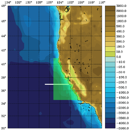
The WC13 model domain is shown in Fig. 1 and has open boundaries along the northern, western, and southern edges of the model domain.
In the tutorial, you will perform a 4D-Var data assimilation cycle that spans the period 3-6 January, 2004. The 4D-Var control vector δz is comprised of increments to the initial conditions, δx(t0), surface forcing, δf(t), and open boundary conditions, δb(t). The prior initial conditions, xb(t0), are taken from the sequence of 4D-Var experiments described by Moore et al. (2011b) in which data were assimilated every 7 days during the period July 2002- December 2004. The prior surface forcing, fb(t), takes the form of surface wind stress, heat flux, and a freshwater flux computed using the ROMS bulk flux formulation, and using near surface air data from COAMPS (Doyle et al., 2009). Clamped open boundary conditions are imposed on (u,v) and tracers, and the prior boundary conditions, bb(t), are taken from the global ECCO product (Wunsch and Heimbach, 2007). The free-surface height and vertically integrated velocity components are subject to the usual Chapman and Flather radiation conditions at the open boundaries. The prior surface forcing and open boundary conditions are provided daily and linearly interpolated in time. Similarly, the increments δf(t) and δb(t) are also computed daily and linearly interpolated in time.
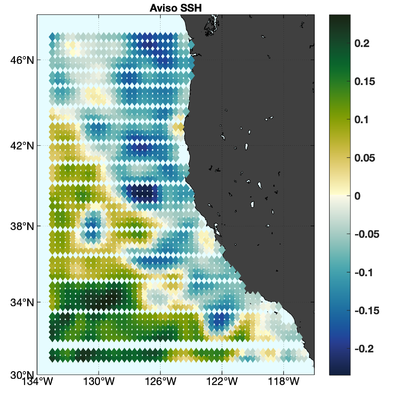
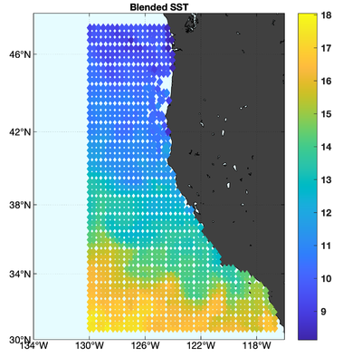
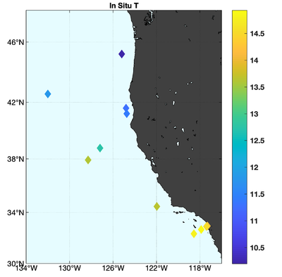
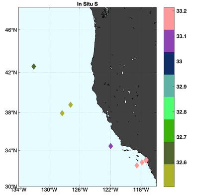
The observations assimilated into the model are satellite SST, satellite SSH in the form of a gridded product from Aviso, and hydrographic observations of temperature and salinity collected from Argo floats and during the GLOBEC/LTOP and CalCOFI cruises off the coast of Oregon and southern California, respectively. The observation locations are illustrated in Fig. 2.
 |
 |
 |
 |
Running 4D-PSAS
To run this tutorial, go first to the directory WC13/PSAS. Instructions for compiling and running the model are provided below or can be found in the Readme file. The recommended configuration for this exercise is one outer-loop and 50 inner-loops, and roms_wc13.in is configured for this default case. The number of inner-loops is controlled by the parameter Ninner in roms_wc13.in.
Important CPP Options
The following C-preprocessing options are activated in the build script:
POSTERIOR_EOFS Estimate posterior analysis error
POSTERIOR_ERROR_I Estimate initial posterior analysis error
WC13 Application CPP option
Input NetCDF Files
WC13 requires the following input NetCDF files:
Nonlinear Initial File: wc13_ini.nc
Forcing File 01: ../Data/coamps_wc13_lwrad_down.nc
Forcing File 02: ../Data/coamps_wc13_Pair.nc
Forcing File 03: ../Data/coamps_wc13_Qair.nc
Forcing File 04: ../Data/coamps_wc13_rain.nc
Forcing File 05: ../Data/coamps_wc13_swrad.nc
Forcing File 06: ../Data/coamps_wc13_Tair.nc
Forcing File 07: ../Data/coamps_wc13_wind.nc
Boundary File: ../Data/wc13_ecco_bry.nc
Initial Conditions STD File: ../Data/wc13_std_i.nc
Model STD File: ../Data/wc13_std_m.nc
Boundary Conditions STD File: ../Data/wc13_std_b.nc
Surface Forcing STD File: ../Data/wc13_std_f.nc
Initial Conditions Norm File: ../Data/wc13_nrm_i.nc
Model Norm File: ../Data/wc13_nrm_m.nc
Boundary Conditions Norm File: ../Data/wc13_nrm_b.nc
Surface Forcing Norm File: ../Data/wc13_nrm_f.nc
Observations File: wc13_obs.nc
Various Scripts and Include Files
The following files will be found in WC13/PSAS directory after downloading from ROMS test cases SVN repository:
build_roms.bash bash shell script to compile application
build_roms.sh csh Unix script to compile application
job_psas.sh job configuration script
roms_wc13.in ROMS standard input script for WC13
s4dvar.in 4D-Var standard input script template
wc13.h WC13 header with CPP options
Instructions
To run this application you need to take the following steps:
- We need to run the model application for a period that is long enough to compute meaningful circulation statistics, like mean and standard deviations for all prognostic state variables (zeta, u, v, T, and S). The standard deviations are written to NetCDF files and are read by the 4D-Var algorithm to convert modeled error correlations to error covariances. The error covariance matrix, D=diag(Bx, Bb, Bf, Q), is very large and not well known. B is modeled as the solution of a diffusion equation as in Weaver and Courtier (2001). Each covariance matrix is factorized as B = K Σ C ΣT KT, where C is a univariate correlation matrix, Σ is a diagonal matrix of error standard deviations, and K is a multivariate balance operator.In this application, we need standard deviations for initial conditions, surface forcing (ADJUST_WSTRESS and ADJUST_STFLUX), and open boundary conditions (ADJUST_BOUNDARY). The standard deviations for the initial and open boundary conditions are in terms of the unbalanced error covariance (K Bu KT) since the balanced operator is activated (BALANCE_OPERATOR and ZETA_ELLIPTIC).The balance operator imposes a multivariate constraint on the error covariance such that the unobserved variable information is extracted from observed data by establishing balance relationships (i.e., T-S empirical formulas, hydrostactic balance, and geostrophic balance) with other state variables (Weaver et al., 2005).These standard deviations have already been created for you:../Data/wc13_std_i.nc initial conditions
../Data/wc13_std_m.nc model error (if weak constraint)
../Data/wc13_std_b.nc open boundary conditions
../Data/wc13_std_f.nc surface forcing (wind stress and net heat flux) - Since we are modeling the error covariance matrix, D, we need to compute the normalization coefficients to ensure that the diagonal elements of the associated correlation matrix C are equal to unity. There are two methods to compute normalization coefficients: exact and randomization (an approximation).The exact method is very expensive on large grids. The normalization coefficients are computed by perturbing each model grid cell with a delta function scaled by the area (2D state variables) or volume (3D state variables), and then by convolving with the squared-root adjoint and tangent linear diffusion operators.The approximate method is cheaper: the normalization coefficients are computed using the randomization approach of Fisher and Courtier (1995). The coefficients are initialized with random numbers having a uniform distribution (drawn from a normal distribution with zero mean and unit variance). Then, they are scaled by the inverse squared-root of the cell area (2D state variable) or volume (3D state variable) and convolved with the squared-root adjoint and tangent diffusion operators over a specified number of iterations, Nrandom.Check following parameters in the 4D-Var input script s4dvar.in (see input script for details):Nmethod == 0 ! normalization methodThese normalization coefficients have already been computed for you (../Normalization) using the exact method since this application has a small grid (54x53x30):
Nrandom == 5000 ! randomization iterations
LdefNRM == F F F F ! Create a new normalization files
LwrtNRM == F F F F ! Compute and write normalization
CnormI(isFsur) = T ! 2D variable at RHO-points
CnormI(isUbar) = T ! 2D variable at U-points
CnormI(isVbar) = T ! 2D variable at V-points
CnormI(isUvel) = T ! 3D variable at U-points
CnormI(isVvel) = T ! 3D variable at V-points
CnormI(isTvar) = T T ! NT tracers
CnormB(isFsur) = T ! 2D variable at RHO-points
CnormB(isUbar) = T ! 2D variable at U-points
CnormB(isVbar) = T ! 2D variable at V-points
CnormB(isUvel) = T ! 3D variable at U-points
CnormB(isVvel) = T ! 3D variable at V-points
CnormB(isTvar) = T T ! NT tracers
CnormF(isUstr) = T ! surface U-momentum stress
CnormF(isVstr) = T ! surface V-momentum stress
CnormF(isTsur) = T T ! NT surface tracers flux../Data/wc13_nrm_i.nc initial conditionsNotice that the switches LdefNRM and LwrtNRM are all false (F) since we already computed these coefficients.
../Data/wc13_nrm_m.nc model error (if weak constraint)
../Data/wc13_nrm_b.nc open boundary conditions
../Data/wc13_nrm_f.nc surface forcing (wind stress and
net heat flux)The normalization coefficients need to be computed only once for a particular application provided that the grid, land/sea masking (if any), and decorrelation scales (HdecayI, VdecayI, HdecayB, VdecayV, and HdecayF) remain the same. Notice that large spatial changes in the normalization coefficient structure are observed near the open boundaries and land/sea masking regions. - Customize your preferred build script and provide the appropriate values for:
- Root directory, MY_ROOT_DIR
- ROMS source code, MY_ROMS_SRC
- Fortran compiler, FORT
- MPI flags, USE_MPI and USE_MPIF90
- Path of MPI, NetCDF, and ARPACK libraries according to the compiler. Notice that you need to provide the correct places of these libraries for your computer. If you want to ignore this section, comment out the assignment for the variable USE_MY_LIBS.
- Notice that the most important CPP options for this application are specified in the build script instead of wc13.h:setenv MY_CPP_FLAGS "-DW4DPSAS"This is to allow flexibility with different CPP options.
setenv MY_CPP_FLAGS "${MY_CPP_FLAGS} -DPOSTERIOR_EOFS"
setenv MY_CPP_FLAGS "${MY_CPP_FLAGS} -DPOSTERIOR_ERROR_I"For this to work, however, any #undef directives MUST be avoided in the header file wc13.h since it has precedence during C-preprocessing. - You MUST use the build script to compile.
- Customize the ROMS input script roms_wc13.in and specify the appropriate values for the distributed-memory partition. It is set by default to:Notice that the adjoint-based algorithms can only be run in parallel using MPI. This is because of the way that the adjoint model is constructed.
- Customize the configuration script job_psas.sh and provide the appropriate place for the substitute Perl script:set SUBSTITUTE=${ROMS_ROOT}/ROMS/Bin/substituteThis script is distributed with ROMS and it is found in the ROMS/Bin sub-directory. Alternatively, you can define ROMS_ROOT environmental variable in your .cshrc login script. For example, I have:setenv ROMS_ROOT /home/arango/ocean/toms/repository/trunk
- Execute the configuration job_psas.sh before running the model. It copies the required files and creates psas.in input script from template s4dvar.in. This has to be done every time that you run this application. We need a clean and fresh copy of the initial conditions and observation files since they are modified by ROMS during execution.
- Run ROMS with data assimilation:mpirun -np 4 romsM roms_wc13.in > & log &
Plotting your Results
Several Matlab scripts are provided in the directory WC13/plotting which will allow you to plot some of the 4D-PSAS output.
Recall that 4D-PSAS minimizes the cost function given by:
Plot first the 4D-PSAS cost function and its components , and the theoretical minimum value using the Matlab script plot_psas_cost.m.
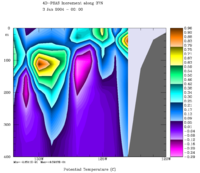
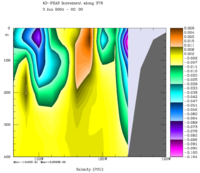
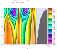
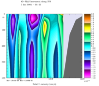
Next, plot the surface initial conditions increments and the surface forcing increments at initial time using Matlab script plot_psas_increments.m or ROMS plotting package script ccnt_psas_increments.in for horizontal plots at 100 m or csec_psas_increments.in for cross-sections along 37°N.
Results
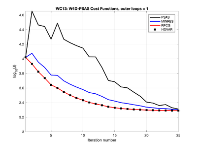
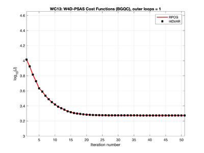
The 4D-PSAS cost function value for each inner loop iteration is shown below:
 |
 |
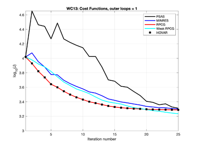 |
The total cost function J (black curve), observation cost function Jo (blue curve), and background cost function Jb (red curve) are plotted on a log10 scale. The value of the nonlinear cost function JNL at the end of the inner loops is also shown (red X). The horizontal, dashed line shows the theoretical Jmin.
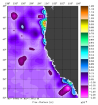
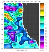
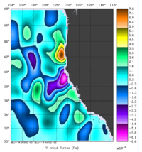
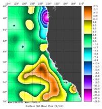
The 4D-PSAS initial conditions increments for free-surface (m), surface wind stress components (Pa), and surface net heat flux (W/m2) are shown below:
 |
 |
 |
 |
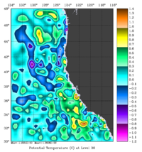
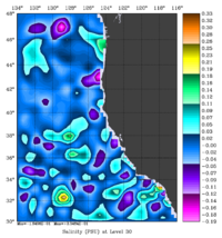
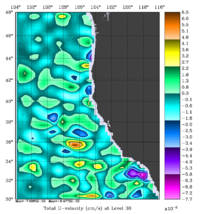
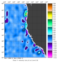
The 4D-PSAS initial conditions increments at the surface for temperature (°C), salinity, and momentum components (m/s) are shown below:
 |
 |
 |
 |
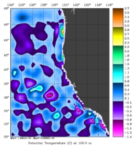
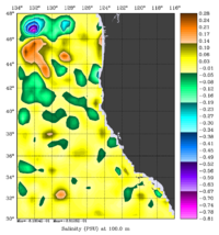
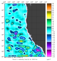
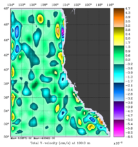
The 4D-PSAS initial conditions increments at 100m for temperature (°C), salinity, and momentum components (m/s) are shown below:
 |
 |
 |
 |
A cross-section along 37°N for the 4D-PSAS initial conditions increments is shown below.
 |
 |
 |
 |


