Vertical S-coordinate
<wikitex> ROMS has a generalized vertical, terrain-following, coordinate system. Currently, two vertical transformation equations, $z=z(x,y,\sigma,t)$, are available which can support numerous vertical stretching 1D-functions when several constraints are satisfied. </wikitex>
Transformation Equations
<wikitex> The following vertical coordinate transformations are available: $$ \eqalign {
     z(x,y,\sigma,t) &= S(x,y,\sigma) + \zeta(x,y,t) \left[1 + \frac{S(x,y,\sigma)}{h(x,y)}\right], \cr
  \noalign{\medskip}
       S(x,y,\sigma) &= h_c \, \sigma + \left[h(x,y) - h_c\right] \, C(\sigma) } \eqno{(1)} $$
or $$ \eqalign {
     z(x,y,\sigma,t) &= \zeta(x,y,t) + \left[\zeta(x,y,t) + h(x,y)\right] \, S(x,y,\sigma), \cr
  \noalign{\medskip}
       S(x,y,\sigma) &= \frac{h_c \, \sigma + h(x,y)\, C(\sigma)}{h_c + h(x,y)} } \eqno{(2)} $$
where $S(x,y,\sigma)$ is a nonlinear vertical transformation functional, $\zeta(x,y,t)$ is the time-varying free-surface, $h(x,y)$ is the unperturbed water column thickness and $z=-h(x,y)$ corresponds to the ocean bottom, $\sigma$ is a fractional vertical stretching coordinate ranging from $-1 \le\sigma\le 0$, $C(\sigma)$ is a nondimensional, monotonic, vertical stretching function ranging from $-1 \le C(\sigma) \le 0$, and $h_c$ is a positive thickness controlling the stretching. In sediment applications, $h=h(x,y,t)$ is changed at every time-step since it is affected by erosion and deposition processes.
![]() Warning: We are now very strict about the value of $h_{c}$ and other input vertical transformation parameters. Since the beginning of ROMS, $h_c=\min(h_{min},T_{cline})$ where $h_{min}\equiv\hbox{minval}(h)$ and $T_{cline}$ is the stretching parameter specified in ocean.in. Notice that it is not possible to build the vertical stretching coordinates when $h_{c}> h_{min}$ and using transformation (1) because it yields $\partial{z}/\partial{\sigma} < 0$ . This has been a legacy issue in ROMS for years, and you are either consistent with the previous set-up of your application or change the value of $T_{cline}$ in all input NetCDF files and ocean.in. Therefore, in new applications you need to be sure that $T_{cline} \le h_{min}$ when using the transformation (1). Notice that this restriction is removed in transformation (2) and $h_c$ can be any positive value. It works for both $h_c \le h_{min}$ or $h_c > h_{min}$ . Again, we are now checking internally for all stretching parameters for consistency in all input NetCDF files that have such variables.
Warning: We are now very strict about the value of $h_{c}$ and other input vertical transformation parameters. Since the beginning of ROMS, $h_c=\min(h_{min},T_{cline})$ where $h_{min}\equiv\hbox{minval}(h)$ and $T_{cline}$ is the stretching parameter specified in ocean.in. Notice that it is not possible to build the vertical stretching coordinates when $h_{c}> h_{min}$ and using transformation (1) because it yields $\partial{z}/\partial{\sigma} < 0$ . This has been a legacy issue in ROMS for years, and you are either consistent with the previous set-up of your application or change the value of $T_{cline}$ in all input NetCDF files and ocean.in. Therefore, in new applications you need to be sure that $T_{cline} \le h_{min}$ when using the transformation (1). Notice that this restriction is removed in transformation (2) and $h_c$ can be any positive value. It works for both $h_c \le h_{min}$ or $h_c > h_{min}$ . Again, we are now checking internally for all stretching parameters for consistency in all input NetCDF files that have such variables.
We find it convenient to define:
$$ H_z \equiv {\partial z \over \partial \sigma} $$
where $H_z=H_z(x,y,\sigma,t)$ are the vertical grid thicknesses. In ROMS, $H_z$ is computed discretely as $\Delta z/ \Delta \sigma$ since this leads to the vertical sum of $H_z$ being exactly the total water column thickness $D$.
![]() Transformation (1) has been available in ROMS since 1999. It is activated by setting Vtransform = 1 in ocean.in. Notice that,
Transformation (1) has been available in ROMS since 1999. It is activated by setting Vtransform = 1 in ocean.in. Notice that,
$$ S(x,y,\sigma) = \cases{0,        &if $\;\;\sigma = \phantom{-}0,  \;\; C(\sigma) = \phantom{-}0, \qquad\hbox{at the free-surface;}$\cr
                          -h(x,y),  &if $\;\;\sigma = -1, \;\; C(\sigma) = -1$, \qquad\hbox{at the ocean bottom.}\cr}$$
In an undisturbed ocean state, corresponding to zero free-surface, $z=S(x,y,\sigma)$. Shchepetkin and McWilliams (2005) denotes this transformation as an unperturbed coordinate system since all the depths are not affected by the displacements of the free-surface. This ensures that the vertical mass fluxes generated by a purely barotropic motion will vanish at every interface
![]() Transformation (2) has been available in UCLA-ROMS since 2005. It is activated by setting Vtransform = 2 in ocean.in. Notice that,
Transformation (2) has been available in UCLA-ROMS since 2005. It is activated by setting Vtransform = 2 in ocean.in. Notice that,
$$ S(x,y,\sigma) = \cases{0,        &if $\;\;\sigma = \phantom{-}0,  \;\; C(\sigma) = \phantom{-}0, \qquad\hbox{at the free-surface;}$\cr
                          -1,       &if $\;\;\sigma = -1, \;\; C(\sigma) = -1$, \qquad\hbox{at the ocean bottom;}\cr}$$
which is different to the behavior of the original functional in (1). Shchepetkin (personal communication) points out that (2) offers several advantages:
- Regardless of the design of $C(\sigma)$, it behaves like equally-spaced sigma-coordinates in shallow regions, where $h(x,y) \ll h_c$. This is advantageous because it avoids excessive resolution and associated CFL limitation is such areas.
- Near-surface refinement behaves more or less like geopotential coordinates in deep regions (level thicknesses, $H_z$, do not depend or weakly depend on bathymetry), while near-bottom like sigma coordinates ($H_z$ is roughly proportional to depth). This reduces the extreme r-factors near the bottom and reduces pressure gradient errors.
- The true sigma-coordinate system is recovered as $h_c \rightarrow \infty$. This is useful when configuring applications with flat bathymetry and uniform level thickness. Practically, you can achieve this by setting Tcline to 1.0d+16 in ocean.in. This will set $h_c=1.0\hbox{x}10^{16}$. Although not necessary, we also recommend that you set $\theta_S=0$ and $\theta_B=0$.
In an undisturbed ocean state, $\zeta\equiv 0$, transformation (2) yields the following unperturbed depths, $\hat{z}$,
$$ \hat{z}(x,y,\sigma) \equiv h(x,y) \, S(x,y,\sigma) = h(x,y) \left[\frac{h_c \, \sigma + h(x,y)\, C(\sigma)}{h_c + h(x,y)}\right] \eqno{(3)} $$
and
$$ d\hat{z} = d\sigma \; h(x,y) \; \left[\frac{h_c}{h_c + h(x,y)}\right] \eqno{(4)} $$
As a consequence, the uppermost grid box retains very little dependency from bathymetry in deep areas, where $h_c \ll h(x,y)$. For example, if $h_c = 250\,m$ and $h(x,y)$ changes from $2000$ to $6000\,m$, the uppermost grid box changes only by a factor of 1.08 (less than $10\%$). </wikitex>
Vertical Stretching Functions
<wikitex> The above generic vertical transformation design facilitates numerous vertical stretching functions, $C(\sigma)$. This function is defined in terms of several parameters which are specified in the standard input file, ocean.in.
Stretching Function Properties:
- $C(\sigma)$ is a dimensionless, nonlinear, monotonic function;
- $C(\sigma)$ is a continuous differentiable function, or a differentiable piecewise function with smooth transition;
- $C(\sigma)$ must be discritized in terms of the fractional stretched vertical coordinate $\sigma$,
 $$ \sigma(k) = \cases{\frac{k-N}{N},        &at vertical $W\hbox{-points},    \;k=0,\dots,N$, \cr\cr
                       \frac{k-N-0.5}{N},    &at vertical $\rho\hbox{-points}, \;\;\;k=1,\dots,N$  \cr}$$
- $C(\sigma)$ must be constrained by $-1 \le C(\sigma) \le 0$, that is,
$$ C(\sigma) = \cases{0,        &for $\;\;\sigma = \phantom{-}0,  \qquad\hbox{at the free-surface;}$\cr
                      -1,       &for $\;\;\sigma = -1, \qquad\hbox{at the ocean bottom.}$\cr}$$
Available Stretching Functions:
- Song and Haidvogel (1994) function available in ROMS since its beginning, Vstretching = 1. $C(\sigma)$ is defined as:
$$C(\sigma) = (1 - \theta_B) {\sinh (\theta_S\,\sigma) \over \sinh \theta_S } + \theta_B \left[{ \tanh [\theta_S ( \sigma + {1\over 2})] \over 2 \tanh ( {1\over 2} \theta_S) } - \frac{1}{2}\right] \eqno{(5)} $$
where ${\theta_S}$ and $\theta_B$ are the surface and bottom control parameters. Their ranges are $0 < \theta_S \leq 20$ and $0 \leq \theta_B \leq 1$, respectively. This function has the following features:- It is infinitely differentiable in $\sigma$.
- The larger the value of ${\theta_S}$, the more resolution is kept above $h_c$.
- For $\theta_B = 0$, the resolution all goes to the surface as $\theta_S$ is increased.
- For $\theta_B = 1$, the resolution goes to both the surface and the bottom equally as $\theta_S$ is increased.
- For $\theta_S \neq 0$, there is a subtle mismatch in the discretization of the model equations, for instance in the horizontal viscosity term. We recommend that you stick with reasonable values of $\theta_S$, say $\theta_S \leq 8$.
- Some applications turn out to be sensitive to the value of $\theta_S$ used.
- A. Shchepetkin (2005) UCLA-ROMS deprecated function, Vstretching = 2. $C(\sigma)$ is defined as a piecewise function:
$$ C(\sigma) = \mu \, C_{sur}(\sigma) + (1 - \mu) \, C_{bot}(\sigma), $$ $$ C_{sur}(\sigma) = \frac{1 - \cosh(\theta_S \, \sigma)}{\cosh(\theta_S) - 1}, \qquad \hbox{for }\theta_S > 0, \qquad C_{bot}(\sigma) = \frac{\sinh[\theta_B \,(\sigma + 1)]}{\sinh(\theta_B)} - 1, \qquad \hbox{for }\theta_B > 0, \eqno{(6)} $$ $$ \mu = (\sigma + 1)^{\alpha} \; \left[1 + \frac{\alpha}{\beta} \left(1 - (\sigma + 1)^{\beta}\right)\right] $$ This function is similar in meaning to the Song and Haidvogel (1994), but note that hyperbolic function in $C_{sur}$ is $\cosh$ instead of $\sinh$ and
$$ \frac {\partial C}{\partial\sigma} \rightarrow 0 \qquad \hbox{as} \;\;\sigma \rightarrow 0.$$ - R. Geyer function for high bottom boundary layer resolution in relatively shallow applications, Vstretching = 3. $C(\sigma)$ is defined as a piecewise function:
$$ C(\sigma) = \mu \, C_{bot}(\sigma) + (1 - \mu) \, C_{sur}(\sigma), $$ $$ C_{sur}(\sigma) = - \frac{\log[\cosh(\gamma\,\hbox{abs}(\sigma)^{\theta_S}] }{\log[\cosh(\gamma)]}, \qquad C_{bot}(\sigma) = \frac{\log[\cosh(\gamma\,(\sigma+1)^{\theta_B}]}{\log[\cosh(\gamma)]} - 1, \eqno{(7)} $$ $$ \mu = \frac{1}{2} \left[1 - \tanh\left(\gamma\left(\sigma + \frac{1}{2}\right)\right)\right] $$ where the power exponents ${\theta_S}$ and $\theta_B$ are the surface and bottom control parameters specified in standard input file ocean.in, as before. Here, $\gamma$ is a scale factor for all hyperbolic functions. Currently, $\gamma = 3$. Typical values for the control parameters are:
$\theta_S=0.65$ minimal increase of surface resolution $\theta_S=1.0$ significant surface amplification $\theta_B=0.58$ no bottom amplification $\theta_B=1.0$ significant bottom amplification $\theta_B=1.5$ good bottom resolution for gravity flows $\theta_B=3.0$ super-high bottom resolution - A. Shchepetkin (2010) UCLA-ROMS current function, Vstretching = 4. $C(\sigma)$ is defined as a continuous, double stretching function:
Surface refinement function:
$$ C(\sigma) = \frac{1 - \cosh(\theta_S \, \sigma)}{\cosh(\theta_S) - 1}, \qquad \hbox{for }\theta_S > 0, \qquad C(\sigma) = -{\sigma}^{2}, \qquad \hbox{for }\theta_S \le 0 \eqno{(8)} $$
Bottom refinement function:
$$ C(\sigma) = \frac {\exp(\theta_B\,C(\sigma)) - 1} {1 - \exp(-\theta_B)}, \qquad \hbox{for }\theta_B > 0 \eqno{(9)} $$
Notice that the bottom function (9) is the second stretching of an already stretched transform (8). The resulting stretching function is continuous with respect to $\theta_S$ and $\theta_B$ as their values approach zero. The range of meaningful values for $\theta_S$ and $\theta_B$ are:
$$ 0 \le \theta_S \le 10 \qquad \hbox{and} \qquad 0 \le \theta_B \le 4 $$
However, users need to pay attention to extreme r-factor (rx1) values near the bottom.
 Due to its functionality and properties Vtransform = 2 and Vstretching = 4 are now the default values for ROMS.
</wikitex>
Metadata Considerations
The above vertical transformations have been registered with the CF Conventions Committee and the NetCDF-Java group. We expect that it will take some time for the CF Committee to approve them. However, the NetCDF-Java is expected to be coded right away. Two new standard_name variable attributes: ocean_s_coordinate_g1 and ocean_s_coordinate_g2 have been assigned for transformations (1) and (2), respectively. The terms in the definition are associated with file variables by the formula_terms attribute as follows:
Transformation (1):
       double s_rho(s_rho) ;
               s_rho:long_name = "S-coordinate at RHO-points" ;
               s_rho:valid_min = -1. ;
               s_rho:valid_max = 0. ;
               s_rho:positive = "up" ;
               s_rho:standard_name = "ocean_s_coordinate_g1" ;
               s_rho:formula_terms = "s: s_rho C: Cs_r eta: zeta depth: h depth_c: hc" ;
       double s_w(s_w) ;
               s_w:long_name = "S-coordinate at W-points" ;
               s_w:valid_min = -1. ;
               s_w:valid_max = 0. ;
               s_w:positive = "up" ;
               s_w:standard_name = "ocean_s_coordinate_g1" ;
               s_w:formula_terms = "s: s_w C: Cs_w eta: zeta depth: h depth_c: hc" ;
Transformation (2):
       double s_rho(s_rho) ;
               s_rho:long_name = "S-coordinate at RHO-points" ;
               s_rho:valid_min = -1. ;
               s_rho:valid_max = 0. ;
               s_rho:positive = "up" ;
               s_rho:standard_name = "ocean_s_coordinate_g2" ;
               s_rho:formula_terms = "s: s_rho C: Cs_r eta: zeta depth: h depth_c: hc" ;
       double s_w(s_w) ;
               s_w:long_name = "S-coordinate at W-points" ;
               s_w:valid_min = -1. ;
               s_w:valid_max = 0. ;
               s_w:positive = "up" ;
               s_w:standard_name = "ocean_s_coordinate_g2" ;
               s_w:formula_terms = "s: s_w C: Cs_w eta: zeta depth: h depth_c: hc" ;
![]() Notice that the formula_terms are identical for both transformations and are independent of the vertical stretching function used. This metadata conventions allows to process/visualize any NetCDF file generated by ROMS easily and correctly compute the associated vertical grid depths.
Notice that the formula_terms are identical for both transformations and are independent of the vertical stretching function used. This metadata conventions allows to process/visualize any NetCDF file generated by ROMS easily and correctly compute the associated vertical grid depths.
Vertical Grid Examples
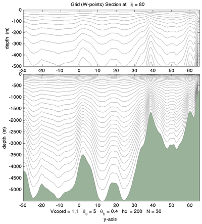
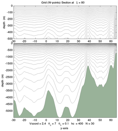
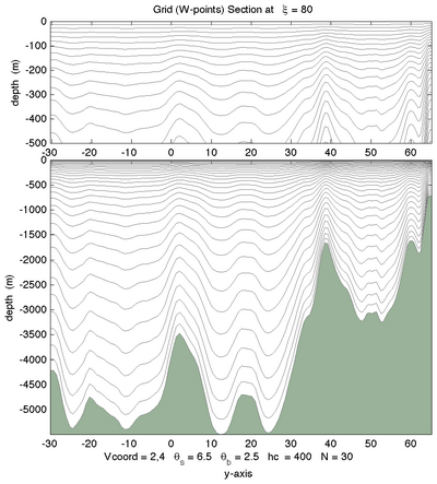
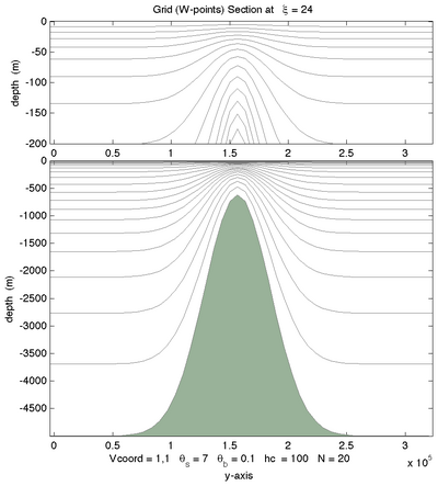
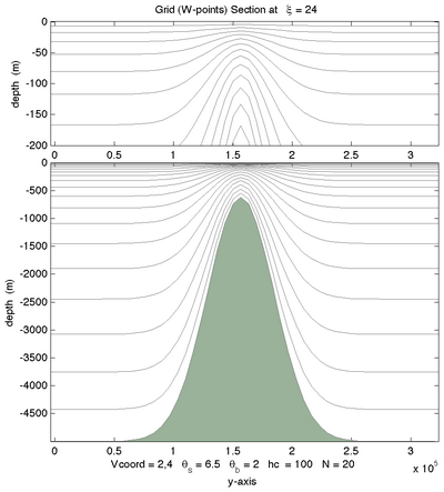
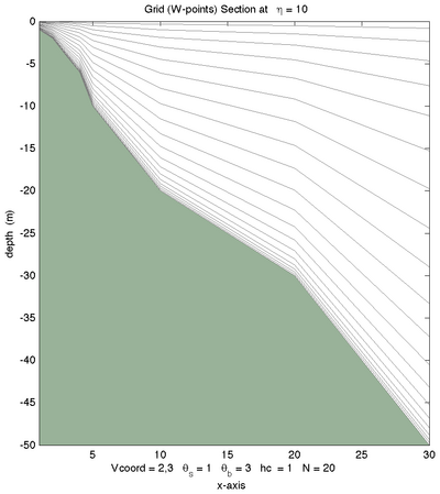
<wikitex> The following figures shows the $\sigma$-surfaces for both vertical transformations and available vertical stretching functions. These plots were generated in Matlab using the script scoord.m.
 |
 |
 |
 |
 |
 |
 |
 |
 |
 |
 |
 |
</wikitex>