Model Coupling
Introduction
The coupling of atmosphere and ocean plays an essential role in the Earth's climate and the long- and short-term predictability of both systems. Typical uncoupled ocean modeling systems utilize atmospheric model data snapshots from files at coarser temporal and spatial resolutions and interpolate the forcing fields at each time step to drive circulation forward. Similarly, some atmospheric modeling systems have simplistic representations of oceanic and air-sea transfer processes. They may use a static sea surface temperature field derived from satellite imagery composited over days to weeks, or one-dimensional ocean mixing models that do not represent three-dimensional baroclinic circulation on continental shelves. This method performs well in regions where the ocean evolves slowly relative to the atmosphere and where the sea state has a limited impact on the atmospheric state. However, in coastal areas, the ocean can respond to the atmosphere rapidly and is highly variable over short spatial scales. In these cases, significant feedbacks between the ocean and atmosphere occur regularly.
Several coupling interfaces exist to exchange data between ESM components including the ESMF (Collins et al., 2005), MCT (Larson et al., 2005), and OASIS (Valcke, 2013) libraries. All three coupling libraries have been used for coupling ROMS with an atmosphere model (e.g., Turuncoglu and Sannino, 2017, Warner et al., 2010, Renault et al., 2016, respectively).
Earth System Modeling Framework (ESMF)
Significant progress has been made over the past decade in the standardization of coupling tools without reducing model diversity through the Earth System Modeling Framework (ESMF; Collins et al., 2005) and the National Unified Operational Prediction Capability (NUOPC) consortia. The NUOPC layer is a simplified infrastructure on top of the ESMF library (version 7 or higher) that provides conventions and templates to facilitate easy coupling between Earth System Models (ESM). It consists of four components: (i) a driver, (ii) the models, (iii) mediators, and (iv) connectors. The driver controls the models, mediators, connectors, and coordinates tasks such as initialization and time stepping. The mediators are custom codes that facilitate the coupling of the models, and control tasks such as flux calculations, rescaling, and averaging. The connectors join ESM components and perform operations such as regridding between the source and destination fields when needed. While the NUOPC layer is available in ESMF version 7 of higher, ROMS coupling requires version 8 or higher because it uses the RunSequence input configuration script and uses version 8 features for nesting.
The critical Fortran module that sits on top of each ESM is the so-called NUOPC cap file. There is a separate cap file for each coupled component, which, from the ROMS perspective, corresponds to the atmosphere, sea-ice, wave model, etc. Therefore, it is an abstract block that allows ROMS to communicate and exchange data seamlessly within the ESMF/NUOPC framework. The ROMS and other ESM grids may (and usually do) have a different geographical extent and horizontal resolution. So if, for example, the atmosphere component domain is larger than the ROMS domain, it is necessary to provide data from another source to the atmosphere model at all of the surface grid points that lie outside the ROMS domain. Therefore, a DATA component and its cap file is also required for most applications. In this case, SST is exported from ROMS and DATA to the atmosphere component which imports a melded SST field.
The ROMS coupling interface with the ESMF/NUOPC library allows both driver and component methods of operation. In the driver method, it provides all the interfaces needed to couple to other ESM components including the executable driver, NUOPC-based generic ESM component services, model gridded components or NUOPC Model cap files, connectors between components for re-gridding source and destination fields, input scripts, and coupling metadata management. A NUOPC Model cap is a Fortran code layer that sits on top of the ESM component, making calls to the numerical kernel via the initialize, run, and finalize phases. Alternatively, in the component method, the stand-alone ROMS NUOPC cap module is also provided, and it can be adapted and incorporated into other NUOPC-based coupling systems, like the NOAA Environmental Modeling System (NEMS) or the Community Mediator for Earth Prediction Systems (CMEPS).
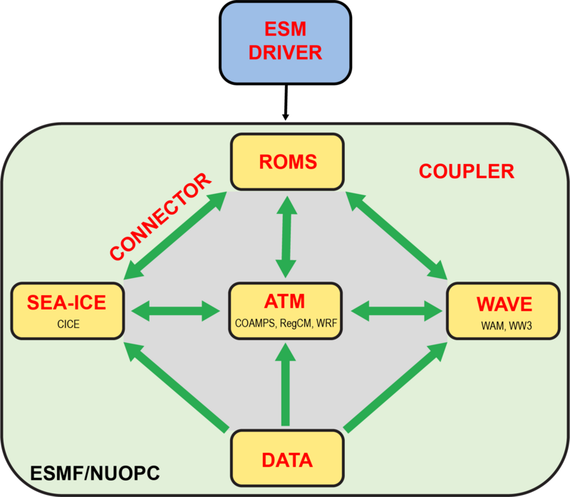
A prototype of the ROMS coupling framework based on the ESMF/NUOPC library is illustrated in Figure 1 showing the Driver, Models, and Connectors. The Driver controls all the aspects of the coupling between the ESM components and their connections: configuration, initialization, time-stepping sequence, data exchanges, and termination. The Models are the gridded data and gridded geophysical numerical kernels wrapped into a NUOPC cap file interface. The Connectors between ESM components execute the remapping and regridding between the source and destination fields. The interpolation is usually linear with extrapolation support in the vicinity of masked grid cells. In the example below, the coupling framework will include an Atmosphere Model, the Ocean Model (ROMS), and the DATA Model since the grids are incongruent. The DATA Model is needed because the Atmosphere Model requires sea surface temperature (SST) on those grid points not covered by ROMS.
Sequential Vs. Concurrent Mode
In sequential mode, all of the coupled model components are executed on all of the processors one after the other sequentially. In concurrent mode, each coupled model component executes on its own set of non-overlapping processors.
Regridding and Extrapolation Methods
Regridding interpolation methods between source and destination fields can be bilinear or conservative. Unmapped cells during regridding are usually located at land/sea boundaries. These unmapped cells can be mapped using the following methods: nearest source to destination, nearest inverse distance average, creep fill at specified level, or two steps extrapolation (Turuncoglu).
# bilinear => bilinear interpolation
# patch => high-order patch recovery
# conservative1 => first-order conservative
# conservative2 => second-order conservative
# nearest => nearest neighbor interpolation
# extrapolate_method Field extrapolation method for unmapped points:
# none => no extrapolation
# nearest => nearest source to destination
# idavg => nearest inverse distance average
# creep => creep fill at specified level
# 2steps => Turuncoglu's 2 steps extrapolation
#
# The ESM imported fields are processed as:
#
# field (destination_units) = field (source_units) * scale + add_offset
ATM_component: &ATM WRF
DATA_component: data.nc
ROMS_component: &OCN ROMS
metadata:
- standard_name: sea_surface_temperature
long_name: sea surface potential temperature
short_name: SST
data_variables: [temperature, time]
source_units: C
destination_units: K
source_grid: cell_center
destination_grid: cell_center
add_offset: 273.15d0
scale: 1.0d0
debug_write: false
connected_to: *ATM
regrid_method: bilinear
extrapolate_method: nearest
- standard_name: sea_surface_temperature_data
long_name: sea surface temperature data
short_name: dSST
data_variables: [temperature, time]
source_units: C
destination_units: K
source_grid: cell_center
destination_grid: cell_center
add_offset: 273.15d0
scale: 1.0d0
debug_write: false
connected_to: *ATM
regrid_method: bilinear
extrapolate_method: nearest
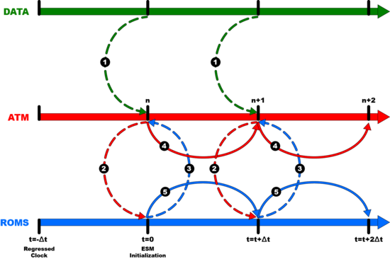
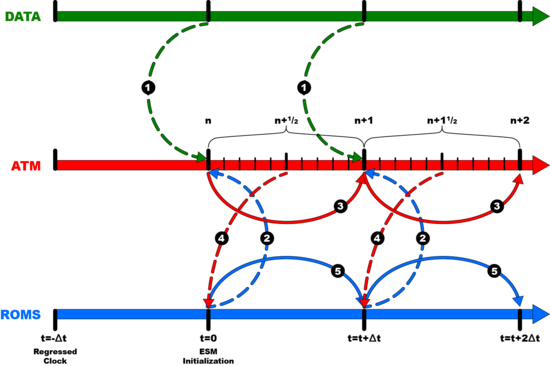
Explicit Vs. Semi-Implicit Run Sequence
|
| |
| Explicit | Semi-Implicit, ATM Average | |
| Atmosphere exports instantaneous fields | Atmosphere exports time-averaged fields
(Recommended for Conservation) |
Semi-Implicit Algorithm Details
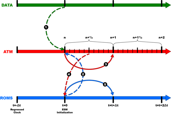
The following diagram shows the sequence of exchanges in a DATA-ATM-ROMS coupling system. The connector ROMS-TO-ATM is explicit, whereas the connector ATM-TO-ROMS is semi-implicit. Usually, the timestep of the atmosphere kernel is smaller than that of the ocean. Thus, ATM export fields are time-averaged over the coupling interval, which is the same as the ROMS timestep. Currently, in our coupling system, we have NUOPC cap files for COAMPS and WRF replacing the generic ATM label.
That is, the detailed sequence of routines called is as follows:
ESM_SetModelServices
ROMS_SetServices
ATM_SetServices
DATA_SetServices
Coupler_SetServices set interpolation RouteHandle ROMS-TO-ATM
Coupler_SetServices set interpolation RouteHandle ATM-TO-ROMS
Coupler_SetServices set interpolation RouteHandle DATA-TO-ATM
ESM_SetRunSequence
ROMS_SetInitializeP1
ATM_SetInitializeP1
DATA_SetInitializeP1
ROMS_SetInitializeP2
ROMS_Initialize
ROMS_SetGridArrays
ROMS_SetStates
ATM_SetInitializeP2
ATM_Initialize
ATM_SetGridArrays
ATM_SetStates
DATA_SetInitializeP2
DATA_Initialize
DATA_multifile
DATA_checkfile
DATA_inquiry
DATA_ncvarcoords
DATA_ncread
DATA_SetGridArrays
DATA_SetStates
Coupler_ComputeRH compute interpolation RouteHandle ROMS-TO-ATM
Coupler_ComputeRH compute interpolation RouteHandle ATM-TO-ROMS
Coupler_ComputeRH compute interpolation RouteHandle DATA-TO-ATM
ROMS_SetClock
ATM_SetClock
DATA_SetClock
ROMS_DataInit
ROMS_Export
ATM_DataInit
Coupler_ExecuteRH apply interpolation RouteHandle DATA-TO-ATM
DATA_ModelAdvance
DATA_ncread
DATA_Export
DATA_TimeInterp
Coupler_ExecuteRH apply interpolation RouteHandle ROMS-TO-ATM
ATM_SetRunClock
ATM_CheckImport
ATM_ModelAdvance
ATM_Import
ATM_ProcessImport
ATM_Export
Coupler_ExecuteRH apply interpolation RouteHandle ATM-TO-ROMS
ROMS_SetRunClock
ROMS_CheckImport
ROMS_ModelAdvance
ROMS_Import
ROMS_Export
Coupler_ExecuteRH apply interpolation RouteHandle DATA-TO-ATM
Coupling with Nested Grids
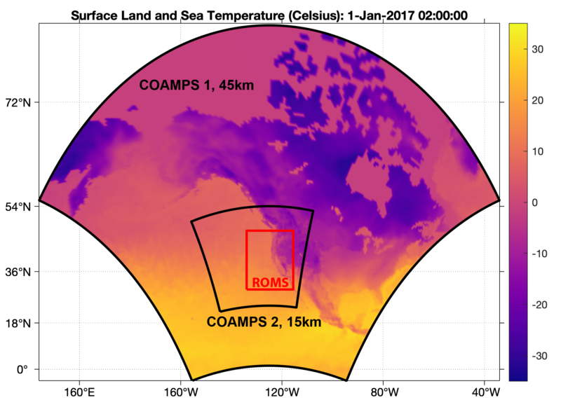
| Component | Grid | CoupledSet | ImportState | ExportState | ConnectedTo |
| ------------------------------------------------------------------------------------------------------------------------------------------------- | |||||
| ROMS | 1 | ESM_02 | Import_ESM_02 | Export_ESM_02 | COAMPS |
| COAMPS | 1 | ESM_01 | Import_ESM_01 | Export_ESM_01 | DATA |
| COAMPS | 2 | ESM_02 | Import_ESM_02 | Export_ESM_02 | ROMS, DATA |
| DATA | 1 | ESM_01 | NONE | Export_ESM_01 | COAMPS |
| DATA | 1 | ESM_02 | NONE | Export_ESM_02 | COAMPS |
- Active coupled Earth System Models (ESM) switches. If a component is nested, each grid is considered an independent component. Specify which nested grids are coupled. The first grid of active ESM components must always be coupled.IsActive(roms) = T ! ROMS (NgridsR)
IsActive(atmos) = T ! atmosphere model (NgridsA)
IsActive(seaice) = F ! seaice model (NgridsI)
IsActive(waves) = F ! wave model (NgridsW)
IsActive(data) = T ! DATA model
- Set which ESM components are connected to the ocean component (ROMS) during coupling. If ROMS has nested grids, indicate which grids are connected to the other ESM components, [1:NgridsR] expected.Coupled(ATM2OCN) == T ! atmosphere -> ROMS connected
Coupled(ICE2OCN) == F ! seaice -> ROMS connected
Coupled(WAV2OCN) == F ! wave -> ROMS connected
Coupled(DAT2OCN) == F ! DATA -> ROMS connected
- Set which ESM components are connected to the atmosphere component during coupling. If the atmosphere component has nested grids, indicate which grids are connected to the other ESM components, [1:NgridsA] expected.Coupled(OCN2ATM) == F T ! ROMS -> atmosphere connected
Coupled(ICE2ATM) == F ! seaice -> atmosphere connected
Coupled(WAV2ATM) == F ! wave -> atmosphere connected
Coupled(DAT2ATM) == T T ! DATA -> atmosphere connected
Model Coupling Toolkit (MCT)
The ROMS modeling system has been coupled to other fully developed models to provide increased modeling capabilites. For the coupling communications, we are using the Model Coupling Toolkit (http://www-unix.mcs.anl.gov/mct/). The original coupling is described in Warner, J.C., Perlin, N., and Skyllingstad, E.D. (2008). Using the Model Coupling Toolkit to couple earth system models, Environmental Modelling & Software, 23, 1240-1249. Since that publication, the coding has been modified to be more generic and allow interfaces to other couplers (such as ESMF).
The coupling provides a mechanism for data transfer between models while they are running concurrently (at the same time). The model coupling requires that each model still needs its own grid, input parameters file, its own time step, forcing files (information not acquired from the other model), and each model writes its own output in its own format (just as if it was not coupled) on its own time interval. However the models are compiled into one executable and exchange information at user defined synchronization intervals.
The current release of ROMS includes 2-way coupling to the wave model SWAN. For coupling to SWAN, the transferred fields are:
 Fields acquired from the WAVE Model:                                !
                                                                     !
    * Dwave      Wave direction.                                     !
    * Hwave      Wave height.                                        !
    * Lwave      Wave length.                                        !
    * Pwave_bot  Wave bottom period.                                 !
    * Pwave_top  Wave surface period.                                !
    * Wave_break Percent of breakig waves.                           !
    * Wave_dissip Wave energy dissipation.                           !
                                                                     !
 Fields sent to the WAVE Model:                                      !
                                                                     !
    * ubar       Depth integrated xi-direction velocity.             !
    * vbar       Depth integrated eta-direction velocity.            !
    * zeta       Water surface elevation.                            !
    * h          Bottom elevation.                                   !
For coupling to the Atmospheric Model WRF, (currently being tested, to be released in the future), the transferred fields are:
 Fields sent to the OCEAN Model:                                     !
                                                                     !
    * PSFC       Surface atmospheric pressure  (mb)                  !
    * RELH       Surface air relative humidity (-)                   !
    * T2         Surface 2m air temperature    (degC)                !
    * U10        U-Wind speed at 10 m          (m/s)                 !
    * V10        V-Wind speed at 10 m          (m/s)                 !
    * CLDFRA     Cloud fraction                (percent/100, so 0-1) !
    * RAIN       Precipitation                 (kg/m2/s)             !
    * SWDOWN     Short wave radiation          (Celsius m/s)         !
    * GLW        Long wave raditaion           (Celsius m/s)         !
    * USTRESS    Surface u-stress              (m2/s2)               !
    * VSTRESS    Surface v-stress              (m2/s2)               !
 Fields acquired from the OCEAN Model:                               !
                                                                     !
    * SST        Sea surface temperature       (degC)                !
The coupling must be compiled with MPI. Users need to first compile the Model Coupling Toolkit, as this library is linked to during the compilation. Examples of coupled applications distributed with the source code include the Tidal Inlet Test Case and the Tidal Headland Test case.
Users need to modify the coupling*.in file to ensure that the correct fields are being transferred. Users should also read the information for the swan.in file.
