Lake Jersey Refinement Example ABD: Difference between revisions
m Text replacement - "ocean_(.*)\.in" to "roms_$1\.in" (change visibility) |
m Text replacement - "\.in" to ".in" (change visibility) |
||
| Line 9: | Line 9: | ||
The Lake Jersey test case is primarily used to evaluate the nesting algorithms for the Refinement Grids Super-Class. It is activated with C-preprocessing options [[Options#LAKE_JERSEY|LAKE_JERSEY]] and [[Options#NESTING|NESTING]]. The nesting algorithms in ROMS are two-way by default. The option [[Options#ONE_WAY|ONE_WAY]] can be used for just one-way exchange between donor ('''dg''') and receiver ('''rg''') grids. However, the one-way exchange has no effect whatsoever on the coarser donor grid because there is no feed back of information. Notice that due to its higher spatial and temporal resolutions, the finer grid is better resolving the physical phenomena at smaller scales. | The Lake Jersey test case is primarily used to evaluate the nesting algorithms for the Refinement Grids Super-Class. It is activated with C-preprocessing options [[Options#LAKE_JERSEY|LAKE_JERSEY]] and [[Options#NESTING|NESTING]]. The nesting algorithms in ROMS are two-way by default. The option [[Options#ONE_WAY|ONE_WAY]] can be used for just one-way exchange between donor ('''dg''') and receiver ('''rg''') grids. However, the one-way exchange has no effect whatsoever on the coarser donor grid because there is no feed back of information. Notice that due to its higher spatial and temporal resolutions, the finer grid is better resolving the physical phenomena at smaller scales. | ||
This example is a refinement application with three grids: coarse ('''a''') and two fine grids('''b''' and '''d'''). There are four contact regions ('''cr''') and two nesting layers because two different time-step sizes are required in <span class="forestGreen">roms_lake_jersey_nested_3g_abd | This example is a refinement application with three grids: coarse ('''a''') and two fine grids('''b''' and '''d'''). There are four contact regions ('''cr''') and two nesting layers because two different time-step sizes are required in <span class="forestGreen">roms_lake_jersey_nested_3g_abd.in</span>: | ||
Latest revision as of 17:35, 8 January 2021
| Example Menu |
|---|
| 1. Introduction |
| 2. Lake Jersey AB |
| 4. Lake Jersey AC |
| 3. Lake Jersey AD |
| 5. Lake Jersey ABD |
| 7. Lake Jersey ADE |
| 6. Lake Jersey ABDC |
| 8. Lake Jersey ACDE |
Description
The Lake Jersey test case is primarily used to evaluate the nesting algorithms for the Refinement Grids Super-Class. It is activated with C-preprocessing options LAKE_JERSEY and NESTING. The nesting algorithms in ROMS are two-way by default. The option ONE_WAY can be used for just one-way exchange between donor (dg) and receiver (rg) grids. However, the one-way exchange has no effect whatsoever on the coarser donor grid because there is no feed back of information. Notice that due to its higher spatial and temporal resolutions, the finer grid is better resolving the physical phenomena at smaller scales.
This example is a refinement application with three grids: coarse (a) and two fine grids(b and d). There are four contact regions (cr) and two nesting layers because two different time-step sizes are required in roms_lake_jersey_nested_3g_abd.in:
- Number of nested grids.Ngrids = 3
- Number of grid nesting layers. This parameter is used to allow refinement and composite grid combinations.NestLayers = 2
- Number of grids in each nesting layer, [1:NestLayers] values are expected.GridsInLayer = 1 2
- Time-stepping parameters.
- Input NetCDF file names, [1:Ngrids] values are expected. The order of the grids are extremely important in nesting applications.
- Nesting grids connectivity data: contact points information. This NetCDF file is special and complex. It is currently generated using the script matlab/grid/contact.m from the Matlab repository.NGCNAME = ../Data/lake_jersey_ngc_3g_abd.nc
- Notice that since the coarse grid (a) is an enclosed basin, all lateral boundary conditions on that grid are set to closed (Clo) while the refined grids (b abd d), which are entirely enclosed by the coarse grid, have nested (Nes) lateral boundary conditions.LBC(isFsur) == Clo Clo Clo Clo \ ! free-surface, Grid 1
Nes Nes Nes Nes \ ! free-surface, Grid 2
Nes Nes Nes Nes ! free-surface, Grid 3
LBC(isUbar) == Clo Clo Clo Clo \ ! 2D U-momentum, Grid 1
Nes Nes Nes Nes \ ! 2D U-momentum, Grid 2
Nes Nes Nes Nes ! 2D U-momentum, Grid 3
LBC(isVbar) == Clo Clo Clo Clo \ ! 2D V-momentum, Grid 1
Nes Nes Nes Nes \ ! 2D V-momentum, Grid 2
Nes Nes Nes Nes ! 2D V-momentum, Grid 3
LBC(isUvel) == Clo Clo Clo Clo \ ! 3D U-momentum, Grid 1
Nes Nes Nes Nes \ ! 3D U-momentum, Grid 2
Nes Nes Nes Nes ! 3D U-momentum, Grid 3
LBC(isVvel) == Clo Clo Clo Clo \ ! 3D V-momentum, Grid 1
Nes Nes Nes Nes \ ! 3D V-momentum, Grid 2
Nes Nes Nes Nes ! 3D V-momentum, Grid 3
LBC(isMtke) == Clo Clo Clo Clo \ ! mixing TKE, Grid 1
Nes Nes Nes Nes \ ! mixing TKE, Grid 2
Nes Nes Nes Nes ! mixing TKE, Grid 3
LBC(isTvar) == Clo Clo Clo Clo \ ! temperature, Grid 1
Clo Clo Clo Clo \ ! salinity, Grid 1
Nes Nes Nes Nes \ ! temperature, Grid 2
Nes Nes Nes Nes \ ! salinity, Grid 2
Nes Nes Nes Nes \ ! temperature, Grid 3
Nes Nes Nes Nes ! salinity, Grid 3
The following tables summarize the nested grids information:
| Grid Information | |||||
|---|---|---|---|---|---|
| Grid | ng | Mesh Size |
Refinement Factor |
Δx Δy |
dt (s) |
| a | 1 | 100x80x8 | - | 500.0 m | 120.0 |
| b | 2 | 66x99x8 | 1:3 from a | 166.6 m | 40.0 |
| d | 3 | 114x60x8 | 1:3 from a | 166.6 m | 40.0 |
| Contact Region Information | ||
|---|---|---|
| cr | dg | rg |
| 1 | 1 (a) | 2 (b) |
| 2 | 1 (a) | 3 (d) |
| 3 | 2 (b) | 1 (a) |
| 4 | 3 (d) | 1 (a) |
The Nested Grids Connectivity (NGC) input NetCDF file is created in Matlab using the following commands:
 >>  Gnames = {'lake_jersey_grd_a.nc', 'lake_jersey_grd_b.nc', 'lake_jersey_grd_d.nc'};
 >>  Cname  = 'lake_jersey_ngc_3g_abd.nc';
 >>  [S,G] = contact(Gnames, Cname);
This creates several figures with useful information. Users need to download the grid processing scripts from ROMS Matlab repository. This Matlab script is quite complex because the nested connectivity is not trivial and is done outside of ROMS for efficiency. See the following pages for detailed information and diagrams.
Results
The plots below show the results after 2 days of simulation for one-way and two-way nesting configurations. They are plotted with Matlab using the script plot_nesting.m. The refined solutions (grids b and d) are overlayed on top of the coarse grid (a). The color map is rendered using shading flat, meaning there is no interpolation between pixels in the color maps. Click the figure to see a more detailed image. On the resulting page a link to the full resolution image is provided.
The figures below were created in Matlab using the following commands:
 >>  Gnames = {'lake_jersey_grd_a.nc', 'lake_jersey_grd_b.nc', 'lake_jersey_grd_d.nc'};
 >>  Anames = {'lake_jersey_avg_a.nc', 'lake_jersey_avg_b.nc', 'lake_jersey_avg_d.nc'};
 >>  Hnames = {'lake_jersey_his_a.nc', 'lake_jersey_his_b.nc', 'lake_jersey_his_d.nc'};
 >>
 >>  G = grids_structure (Hnames, Hnames);
 >>
 >>  F = plot_nesting (G, Hnames, 'temp', 97, 8, 1, true);
 >>  F = plot_nesting (G, Hnames, 'salt', 97, 8, 1, true);
 >>  F = plot_nesting (G, Hnames, 'zeta', 97, 8, 1, true);
 >>
 >>  F = plot_nesting (G, Anames, 'rvorticity_bar', 97, 8, 1, true);
Again, users need to download these scripts from the ROMS Matlab repository.
- Surface Temperature (Celsius)
-
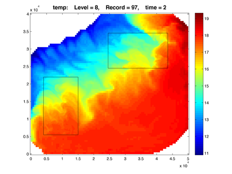
One-way -

Two-way


- Surface Salinity
-
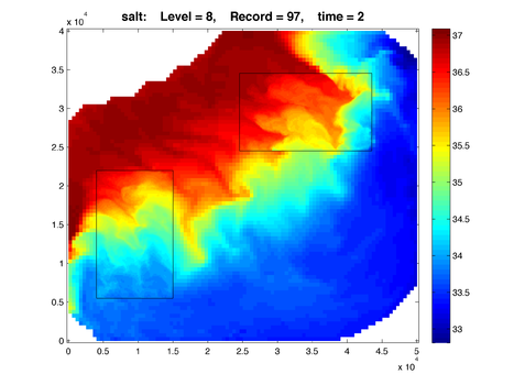
One-way -
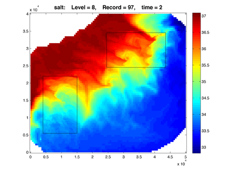
Two-way


- Free-surface (m)
-
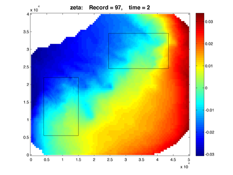
One-way -
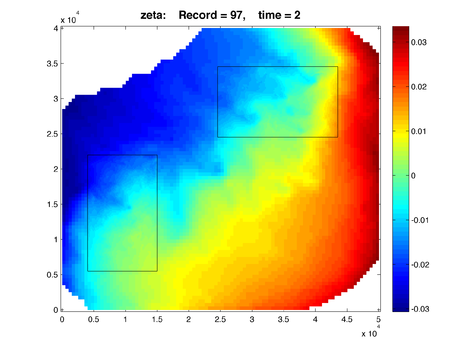
Two-way


- 30-minute Averaged Vertically Integrated Relative Vorticity (1/s)
-
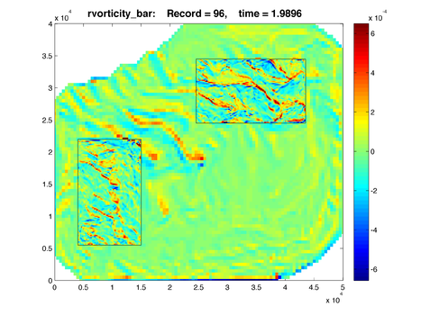
One-way -
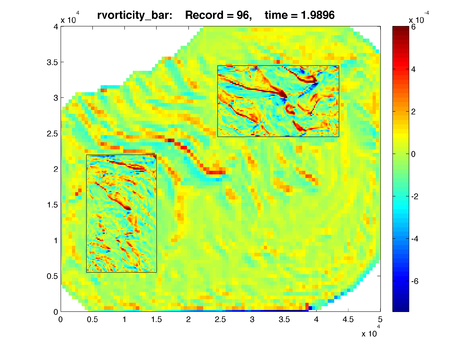
Two-way

