Difference between revisions of "Sea-Ice Model"
(adding some stuff, still not done) (change visibility) |
|||
| (17 intermediate revisions by 2 users not shown) | |||
| Line 1: | Line 1: | ||
<div class="title">Sea-Ice Model</div> | <div class="title">Sea-Ice Model</div> | ||
The sea-ice component of ROMS is a combination of the elastic-viscous-plastic (EVP) rheology ([[Bibliography#HunkeEC_1997a | Hunke and Dukowicz, 1997]], [[Bibliography#HunkeEC_2001a | Hunke, 2001]]) | |||
The sea-ice component of ROMS is a combination of the | and simple one-layer ice and snow thermodynamics with a molecular sublayer under the ice ([[Bibliography#MellorGL_1989a | Mellor and Kantha, 1989]]). It is tightly coupled, having the same grid (Arakawa-C) and timestep as the ocean and sharing the same parallel coding structure for use with MPI or OpenMP. | ||
elastic-viscous-plastic (EVP) rheology ([[Bibliography#HunkeEC_1997a | Hunke and Dukowicz, 1997]], [[Bibliography#HunkeEC_2001a | Hunke, 2001]]) | |||
and simple one-layer ice and snow thermodynamics with a molecular | |||
sublayer under the ice ([[Bibliography#MellorGL_1989a | Mellor and Kantha, 1989]]). It is tightly coupled, having the same grid (Arakawa-C) and timestep as the ocean and sharing the same parallel coding structure for use with MPI or | |||
OpenMP. | |||
__TOC__ | __TOC__ | ||
==Dynamics== | ==Dynamics== | ||
The momentum equations describe the change in ice/snow velocity due | The momentum equations describe the change in ice/snow velocity due | ||
to the combined effects of the Coriolis force, surface ocean tilt, | to the combined effects of the Coriolis force, surface ocean tilt, | ||
air and water stress, and internal ice stress: | air and water stress, and internal ice stress: | ||
<math display="block">\begin{align} | |||
\frac{d}{ dt}(A h_i u) | |||
&= A h_i fv - A h_i g \frac{\partial \zeta_w }{ \partial x} + | |||
\frac{A}{\rho_i}(\tau_a^x + \tau_w^x) + \frac{1}{\rho_i}{\cal F}_x \\ | |||
\frac{d}{ d t}(A h_i v) | |||
&= - A h_i fu - A h_i g \frac{\partial \zeta_w }{ \partial y} + | |||
\frac{A}{\rho_i}(\tau_a^y + \tau_w^y) + \frac{1}{\rho_i}{\cal F}_y\,.\end{align} | |||
</math> | |||
In this model, we neglect the nonlinear advection terms as well as | In this model, we neglect the nonlinear advection terms as well as | ||
the curvilinear terms in the internal ice stress. The force due to | the curvilinear terms in the internal ice stress. Nonlinear formulae are used for both the ocean-ice and air-ice surface stress: | ||
<math display="block">\begin{align} | |||
\vec{\tau}_a &= \rho_a C_a | \vec{V}_{10} | \vec{V}_{10} \\ | |||
C_a &= {1 \over 2} C_d \left[ 1 - \cos( 2 \pi \min(h_i+.1, .5) | |||
\right] \\ | |||
\vec{\tau}_w &= \rho_w C_w | \vec{v}_w - \vec{v} | ( \vec{v}_w - \vec{v})\,.\end{align} | |||
</math> | |||
The force due to | |||
the internal ice stress is given by the divergence of the stress | the internal ice stress is given by the divergence of the stress | ||
tensor | tensor <math>\sigma</math>. The rheology is given by the stress-strain relation of the medium. We would like to emulate the viscous-plastic rheology | ||
of [[Bibliography#HiblerWD_1979a | Hibler (1979)]]: | of [[Bibliography#HiblerWD_1979a | Hibler (1979)]]: | ||
<math display="block">\begin{align} | |||
\sigma_{ij} &= 2 \eta \dot \epsilon_{ij} + (\zeta - \eta) \dot \epsilon_{kk} \delta_{ij} | |||
- {P \over 2} \delta_{ij} \\ | |||
\dot \epsilon_{ij} &\equiv {1 \over 2} \left( {\partial u_i \over \partial x_j} | |||
+ {\partial u_j \over \partial x_i} \right) \end{align} | |||
</math> | |||
where the nonlinear viscosities are given by | |||
<math display="block">\begin{align} | |||
\zeta &= { P \over 2 \left[ (\epsilon^2_{11} + | |||
\epsilon^2_{22} ) ( 1 + 1/e^2 ) + 4 e^{-2} \epsilon^2_{12} | |||
+ 2 \epsilon_{11} \epsilon_{22} ( 1 - 1/e^2 ) \right] ^{1/2} } \\ | |||
\eta &= { \zeta \over e^2 }\,.\end{align} | |||
</math> | |||
Hibler's ice strength is given by: | |||
<math display="block">P = P^* A h_i e^{-C(1-A)}</math> | |||
while [[Bibliography#Overland_1988 | Overland and Pease (1988)]]: advocate a nonlinear strength: | |||
<math display="block">P = P^* A h_i^2 e^{-C(1-A)}</math> | |||
in which <math>P^*</math> now depends on the grid spacing. Both options are available in ROMS. | |||
We would also like to have an explicit model that can be solved | We would also like to have an explicit model that can be solved | ||
efficiently on parallel computers. The EVP rheology has a tunable | efficiently on parallel computers. The EVP rheology has a tunable | ||
coefficient | coefficient <math>E</math> (the Young's modulus) which can be chosen to make the | ||
elastic term small compared to the other terms. We rearrange the VP rheology: | elastic term small compared to the other terms. We rearrange the VP rheology: | ||
<math display="block"> | |||
{1 \over 2 \eta} \sigma_{ij} + {\eta - \zeta \over 4 \eta \zeta} \sigma_{kk} \delta_{ij} | |||
+ {P \over 4 \zeta} \delta_{ij} = \dot \epsilon_{ij} | |||
</math> | |||
then add the elastic term: | then add the elastic term: | ||
<math display="block"> | |||
{1 \over E} {\partial \sigma_{ij} \over \partial t} + {1 \over 2 \eta} \sigma_{ij} | |||
+ {\eta - \zeta \over 4 \eta \zeta} \sigma_{kk} \delta_{ij} | |||
+ {P \over 4 \zeta} \delta_{ij} = \dot \epsilon_{ij} | |||
</math> | |||
Much like the ocean model, the ice model has a split timestep. The | Much like the ocean model, the ice model has a split timestep. The | ||
| Line 56: | Line 80: | ||
allow the elastic wave velocity to be resolved. | allow the elastic wave velocity to be resolved. | ||
Once the new ice velocities are computed, the ice tracers can be advected using the '''MPDATA''' scheme ([[Bibliography#Smolark | Smolarkiewicz]]). The tracers in this case are the ice thickness, ice concentration, snow thickness, internal ice temperature, and surface melt ponds. | Once the new ice velocities are computed, the ice tracers can be advected using the '''MPDATA''' scheme ([[Bibliography#Smolark | Smolarkiewicz]]). The tracers in this case are the ice thickness, ice concentration, snow thickness, internal ice temperature, and surface melt ponds. The continuity equations describing the evolution of these parameters also include thermodynamic terms (<math>S_h</math>, <math>S_s</math> and <math>S_A</math>), described [[#Thermodynamics | below]]: | ||
<math display="block">\begin{align} | |||
{\partial A h_i \over \partial t} &= | |||
- {\partial (u A h_i) \over \partial x} - | |||
{\partial (v A h_i) \over \partial y} | |||
+ S_h + {\cal D}_h \\ | |||
{\partial A h_s \over \partial t} &= | |||
- {\partial (u A h_s) \over \partial x} - | |||
{\partial (v A h_s) \over \partial y} | |||
+ S_s + {\cal D}_s \\ | |||
{\partial A \over \partial t} &= | |||
- {\partial (uA) \over \partial x} - {\partial (vA) \over \partial y} | |||
+ S_A + {\cal D}_A \qquad \qquad 0 \leq A \leq 1\,. \end{align} | |||
</math> | |||
The first two equations represent the conservation of ice and snow. The third is discussed in some detail in [[Bibliography#MellorGL_1989a | Mellor and Kantha, 1989]], but | |||
represents the advection of ice blocks in which no ridging occurs as | |||
long as there is any open water. | |||
The ice model variables: | The ice model variables: | ||
| Line 64: | Line 106: | ||
! Description | ! Description | ||
|- | |- | ||
| | | <math>A(x,y,t)</math> | ||
| | | ice concentration, <math>0.0 \leq A \leq 1.0</math> | ||
|- | |||
| <math>C_a</math> | |||
| nonlinear air drag coefficient | |||
|- | |||
| <math>C_d = 2.2 \times 10^{-3}</math> | |||
| air drag coefficient | |||
|- | |||
| <math>C_w = 10 \times 10^{-3}</math> | |||
| water drag coefficient | |||
|- | |||
| <math>{\cal D}_h, {\cal D}_s, {\cal D}_A</math> | |||
| diffusion terms | |||
|- | |||
| <math>\delta_{ij}</math> | |||
| Kronecker delta function | |||
|- | |||
| <math>E</math> | |||
| Young's modulus | |||
|- | |- | ||
| | | <math>e = 2</math> | ||
| | | eccentricity of the elliptical yield curve | ||
|- | |- | ||
| | | <math>\epsilon_{ij}(x,y,t)</math> | ||
| | | strain rate tensor | ||
|- | |- | ||
| | | <math>\eta(x,y,t)</math> | ||
| | | nonlinear shear viscosity | ||
|- | |- | ||
| | | <math>f(x,y)</math> | ||
| Coriolis parameter | | Coriolis parameter | ||
|- | |- | ||
| | | <math>{\cal F}_x, {\cal F}_y</math> | ||
| | | forces due to internal ice stress | ||
|- | |||
| <math>g</math> | |||
| gravity | |||
|- | |||
| <math>H</math> | |||
| Heaviside function | |||
|- | |- | ||
| | | <math>h_i(x,y,t)</math> | ||
| | | ice thickness | ||
|- | |- | ||
| | | <math>h_o</math> | ||
| | | ice cutoff thickness | ||
|- | |- | ||
| | | <math>h_s(x,y,t)</math> | ||
| | | snow thickness on ice-covered fraction | ||
|- | |- | ||
| | | <math>M</math> | ||
| | | ice mass, <math>\rho_i A h_i</math> | ||
|- | |- | ||
| | | <math>P</math> | ||
| | | ice strength | ||
|- | |- | ||
| | | <math>P^*, C</math> | ||
| | | ice strength parameters | ||
|- | |||
| <math>S_h, S_s, S_A</math> | |||
| thermodynamic terms | |||
|- | |||
| <math>\sigma_{ij}</math> | |||
| internal ice stress tensor | |||
|- | |||
| <math>\vec{\tau}_a</math> | |||
| air stress | |||
|- | |||
| <math>\vec{\tau}_w</math> | |||
| water stress | |||
|- | |- | ||
| | | <math>u,v</math> | ||
| | | the (<math>x,y</math>) components of ice velocity <math>\vec{v}</math> | ||
|- | |- | ||
| | | <math>\vec{V}_{10}, \vec{v}_w</math> | ||
| | | 10 meter air and surface water velocities | ||
|- | |- | ||
| | | <math>\zeta</math> | ||
| | | nonlinear bulk viscosity | ||
|- | |- | ||
| | | <math>\zeta_w</math> | ||
| | | surface elevation of the underlying water | ||
|- | |- | ||
|} | |} | ||
Note that Hibler's <math>h_I</math> variable is | |||
equivalent to our <math>A h_i</math> combination - his <math>h_I</math> is the average | |||
thickness over the whole gridbox while our <math>h_i</math> is the average | |||
equivalent to our | |||
thickness over the whole gridbox while our | |||
thickness over the ice-covered fraction of the gridbox. | thickness over the ice-covered fraction of the gridbox. | ||
==Thermodynamics== | ==Thermodynamics== | ||
The thermodynamics is based on calculating how much ice grows and | The thermodynamics is based on calculating how much ice grows and | ||
melts on each of the surface, bottom, and sides of the ice floes, | melts on each of the surface, bottom, and sides of the ice floes, | ||
as well as frazil ice formation: | as well as frazil ice formation: | ||
[ | [[File:Ice_diag1.png]] | ||
Once the ice tracers are advected, the ice concentration and thickness are timestepped according to the terms on the right: | |||
<math display="block">\begin{align} | |||
\frac{D A h_i}{Dt} &= \frac{\rho_o}{\rho_i} \left[ A (W_{io} - W_{ai}) + (1-A) W_{ao} | |||
+ W_{fr} \right] \\ | |||
\frac{D A}{Dt} &= \frac{\rho_o}{\rho_i h_i} \left[ \Phi (1-A) w_{ao} | |||
+ (1-A) W_{fr} \right] \;\;\;\;\; 0 \leq A \leq 1 \end{align} | |||
</math> | |||
The term <math>Ah_i</math> is the "effective thickness", a measure of the ice volume. Its evolution equation is simply quantifying the change in the amount of ice. The ice concentration equation is more interesting in that | |||
it provides the partitioning between ice melt/growth on the sides vs. on the top and bottom. The parameter <math>\Phi</math> controls this and has differing values for ice melt and retreat. In principle, most of the ice growth is assumed to happen at the base of the ice while rather more of the melt happens on the sides of the ice due to warming of the water in the leads. | |||
The heat fluxes through the ice are based on a simple one layer [[Bibliography#SemtnerAJ_1976a | Semtner (1976)]] type model with snow on top. The temperature is assumed to be linear within the snow and within the ice. The ice contains brine pockets for a total ice salinity of 3.2 or the surface ocean salinity, whichever is less. The surface ocean temperature and salinity is half a <math>dz</math> below the surface. The water right below the surface is assumed to be at the freezing temperature; a logarithmic boundary layer is computed having the temperature and salinity matched at freezing. | |||
Similarly, there is a snow equation: | |||
<math display="block">{D A h_s \over D t} = \left[ A (W_{s} - W_{sm}) \right]</math> | |||
where <math>W_s</math> and <math>W_{sm}</math> are the snowfall and snow melt rates, respectively, in units of equivalent water. Also in the model is the depth of the melt ponds in spring, <math>h_{mp}</math> which can be up to 0.1 m, after which melting ice contributes to <math>W_{ro}</math>. The melt ponds are not part of the thermal conductivity computations. They could contribute to the albedo computation, but that has been largely commented out. | |||
The ice model thermodynamic variables: | |||
{| border="1" cellspacing="0" cellpadding="5" align="center" | |||
! Name | |||
! Description | |||
|- | |||
| <math>\alpha_w = 0.10</math> | |||
| shortwave albedo of water | |||
|- | |||
| <math>\alpha_i = 0.60</math> | |||
| shortwave albedo of wet ice | |||
|- | |||
| <math>\alpha_i = 0.65</math> | |||
| shortwave albedo of dry ice | |||
|- | |||
| <math>\alpha_s</math> | |||
| shortwave albedo of wet snow | |||
|- | |||
| <math>\alpha_s</math> | |||
| shortwave albedo of dry snow | |||
|- | |||
| <math>C_k</math> | |||
| snow correction factor | |||
|- | |||
| <math>C_{pi}</math> = 2093 J kg<math>^{-1}</math> K<math>^{-1}</math> | |||
| specific heat of ice | |||
|- | |||
| <math>C_{po}</math> = 3990 J kg<math>^{-1}</math> K<math>^{-1}</math> | |||
| specific heat of water | |||
|- | |||
| <math>\epsilon_w = 0.97</math> | |||
| longwave emissivity of water | |||
|- | |||
| <math>\epsilon_i = 0.97</math> | |||
| longwave emissivity of ice | |||
|- | |||
| <math>\epsilon_s = 0.99</math> | |||
| longwave emissivity of snow | |||
|- | |||
| <math>E(T,r)</math> | |||
| enthalpy of the ice/brine system | |||
|- | |||
| <math>F_T\!\uparrow</math> | |||
| heat flux from the ocean into the ice | |||
|- | |||
| <math>H\!\downarrow</math> | |||
| sensible heat | |||
|- | |||
| <math>i_w</math> | |||
| fraction of the solar heating transmitted through a lead into the water below | |||
|- | |||
| <math>k_i</math> = 2.04 W m<math>^{-1}</math> K<math>{^-1}</math> | |||
| thermal conductivity of ice | |||
|- | |||
| <math>k_s</math> = 0.31 W m<math>^{-1}</math> K<math>{^-1}</math> | |||
| thermal conductivity of snow | |||
|- | |||
| <math>L_i</math> = 302 MJ m<math>^{-3}</math> | |||
| latent heat of fusion of ice | |||
|- | |||
| <math>L_s</math> = 110 MJ m<math>^{-3}</math> | |||
| latent heat of fusion of snow | |||
|- | |||
| <math>LE\!\downarrow</math> | |||
| latent heat | |||
|- | |||
| <math>LW\!\!\downarrow</math> | |||
| incoming longwave radiation | |||
|- | |||
| <math>m</math> & <math>-0.054^\circ</math>C/PSU | |||
| coefficient in linear <math>T_f(S) = mS</math> equation | |||
|- | |||
| <math>\Phi</math> | |||
| contribution to <math>A</math> equation from freezing water | |||
|- | |||
| <math>Q_{ai}</math> | |||
| heat flux out of the snow/ice surface | |||
|- | |||
| <math>Q_{ao}</math> | |||
| heat flux out of the ocean surface | |||
|- | |||
| <math>Q_{i2}</math> | |||
| heat flux up out of the ice | |||
|- | |||
| <math>Q_{io}</math> | |||
| heat flux up into the ice | |||
|- | |||
| <math>Q_{s}</math> | |||
| heat flux up through the snow | |||
|- | |||
| <math>r</math> | |||
| brine fraction in ice | |||
|- | |||
| <math>\rho_i</math> = 910 <math>m^3/kg</math> | |||
| density of ice | |||
|- | |||
| <math>S_i</math> = 3.2 PSU | |||
| salinity of the ice | |||
|- | |||
| <math>SW\!\!\downarrow</math> | |||
| incoming shortwave radiation | |||
|- | |||
| <math>\sigma</math> = <math>5.67 \times 10^{-8}</math> W m<math>^{-2}</math> K<math>^{-4}</math> | |||
| Stefan-Boltzmann constant | |||
|- | |||
| <math>T_0</math> | |||
| temperature of the bottom of the ice | |||
|- | |||
| <math>T_1</math> | |||
| temperature of the interior of the ice | |||
|- | |||
| <math>T_2</math> | |||
| temperature at the upper surface of the ice | |||
|- | |||
| <math>T_3</math> | |||
| temperature at the upper surface of the snow | |||
|- | |||
| <math>T_f</math> | |||
| freezing temperature | |||
|- | |||
| <math>T_{{\rm melt}\_i}</math> = <math>mS_i</math> | |||
| melting temperature of ice | |||
|- | |||
| <math>T_{{\rm melt}\_s}</math> = 0<math>^\circ</math> C | |||
| melting temperature of snow | |||
|- | |||
| <math>W_{ai}</math> | |||
| melt rate on the upper ice/snow surface | |||
|- | |||
| <math>W_{ao}</math> | |||
| freeze rate at the air/water interface | |||
|- | |||
| <math>W_{fr}</math> | |||
| rate of frazil ice growth | |||
|- | |||
| <math>W_{io}</math> | |||
| freeze rate at the ice/water interface | |||
|- | |||
| <math>W_{ro}</math> | |||
| rate of run-off of surface melt water | |||
|- | |||
| <math>W_{s}</math> | |||
| snowfall rate | |||
|- | |||
| <math>W_{sm}</math> | |||
| snow melt rate | |||
|- | |||
|} | |||
The locations of the ice and snow temperatures and the heat fluxes: | |||
[[File:Ice_diag2.png]] | |||
The temperature profile is assumed to be linear between adjacent temperature points. The interior of the ice contains "brine pockets", leading to a prognostic equation for the temperature <math>T_1</math>. | |||
The surface flux to the air is: | |||
<math display="block"> | |||
Q_{ai} = - H\!\downarrow - LE\!\downarrow - | |||
\epsilon_s LW\!\!\downarrow - | |||
(1 - \alpha_s) SW\!\!\downarrow + \epsilon_s \sigma (T_3+273)^4 | |||
</math> | |||
The incoming shortwave and longwave radiations are assumed to come from an atmospheric model. The formulae for sensible heat, latent heat, and outgoing longwave radiation are the same as in [[Bibliography#ParkinsonCL_1979a |Parkinson and Washington (1979)]] and are shown in [[Radiant Heat Fluxes]]. The sensible heat is a function of <math>T_3</math>, as is the heat flux through the snow <math>Q_s</math>. Setting <math>Q_{ai} = Q_s</math>, we can solve for <math>T_3</math> by setting <math>T_3^{n+1} = T_3^n + \Delta T_3</math> and linearizing in <math>\Delta T_3</math>. As in Parkinson and Washington, if <math>T_3</math> is found to be above the melting temperature, it is set to <math>T_{\rm melt}</math> and the extra energy goes into melting the snow or ice: | |||
<math display="block">\begin{align} | |||
W_{ai} & = \frac{Q_{ai} - Q_{i2} }{ \rho_o L_3} \\ | |||
L_3 & \equiv \left[ E(T_3,1) - E(T_1, R_1) \right]\end{align} | |||
</math> | |||
Note that <math>L_3 = (1-r)L_i</math> plus a small sensible heat correction. We can store water on the surface in melt pools to a fixed depth---everything extra melted at the surface is assumed to flow into the ocean as <math>W_{ro}</math>. The melt ponds however do not contribute to the heat flux computation. | |||
Inside the ice there are brine pockets in which there is salt water at the ''in situ'' freezing temperature. It is assumed that the ice has a uniform overall salinity of <math>S_i</math> and that the freezing temperature is a linear function of salinity. The brine fraction <math>r</math> is given by | |||
<math display="block">r = \frac{S_i m }{ T_1}</math> | |||
The enthalpy of the combined ice/brine system is given by | |||
<math display="block">E(T,r) = r(L_i + C_{po}T) + (1-r) C_{pi} T</math> | |||
Substituting in for <math>r</math> and differentiating gives: | |||
<math display="block"> | |||
\frac{\partial E }{ \partial T} = - \frac{S_i m L_i }{ T_1^2} + C_{pi} | |||
</math> | |||
Inside the snow, we have | |||
<math display="block">Q_s = \frac{k_s }{ h_s} (T_2 - T_3)</math> | |||
The heat conduction in the upper part of the ice layer is | |||
<math display="block">Q_{I2} = \frac{ 2 k_i }{ h_i} (T_1 - T_2)</math> | |||
These can be set equal to each other to solve for <math>T_2</math> | |||
<math display="block">T_2 = \frac{T_3 + C_k T_1 }{ 1 + C_k}</math> | |||
where | |||
<math display="block">C_k \equiv \frac{2 k_i h_s }{ h_i k_s}\,.</math> | |||
Substituting into (\ref{qi2}), we get: | |||
<math display="block"> | |||
Q_s = Q_{I2} = \frac{2k_i }{ h_i} \frac{(T_1 - T_3) }{ (1 + C_k)} | |||
</math> | |||
Note that in the absence of snow, <math>C_k</math> becomes zero and we recover the formula for the no-snow case in which <math>T_3 = T_2</math>. | |||
At the bottom of the ice, we have | |||
The | <math display="block">Q_{I0} = \frac{2 k_i }{ h_i} (T_0 - T_1)</math> | ||
The difference between <math>Q_{I0}</math> and <math>Q_{I2}</math> goes into the enthalpy of the ice: | |||
<math display="block"> | |||
\rho_i h_i \left[ \frac{\partial E }{ \partial t} + \vec{v} \cdot | |||
\nabla E \right] = Q_{I0} - Q_{I2} | |||
</math> | |||
We can use the chain rule to obtain an equation for timestepping <math>T_1</math>: | |||
<math display="block"> | |||
\rho_i h_i \frac{\partial E }{ \partial T} | |||
\left[ \frac{\partial T_1 }{ \partial t} + \vec{v} \cdot | |||
\nabla T_1 \right] = Q_{I0} - Q_{I2} | |||
</math> | |||
where | |||
<math display="block">\begin{align} | |||
Q_{I0} - Q_{I2} & = \frac{2 k_i }{ h_i} \left[ (T_0 - T_1) - | |||
\frac{(T_1 - T_3) }{ 1 + C_k} \right] \\ | |||
& = \frac{2 k_i }{ h_i} \left[ (T_0 + | |||
\frac{T_3 - (2 + C_k) T_1 }{ 1 + C_k} \right]\end{align} | |||
</math> | |||
==Ocean surface boundary conditions== | ==Ocean surface boundary conditions== | ||
==Frazil | The ocean receives surface stresses from both the atmosphere and the ice, according to the ice concentration: | ||
<math display="block">\begin{align} | |||
K_m \frac{\partial u_w }{ \partial z} & = \frac{A }{ \rho_o} \tau_{io}^x | |||
+ \frac{1-A }{ \rho_o} \tau_{ao}^x \\ | |||
K_m \frac{\partial v_w }{ \partial z} & = \frac{A }{ \rho_o} \tau_{io}^y | |||
+ \frac{1-A }{ \rho_o} \tau_{ao}^y \end{align} | |||
</math> | |||
where the relevant variables are in the following table: | |||
{| border="1" cellspacing="0" cellpadding="5" align="center" | |||
! Variable | |||
! Value | |||
! Definition | |||
|- | |||
| <math>b</math> | |||
| 3.14 | |||
| factor | |||
|- | |||
| <math>\dot{E}</math> | |||
| | |||
| evaporation | |||
|- | |||
| <math>k</math> | |||
| 0.4 | |||
| von Karman's constant | |||
|- | |||
| <math>K_m</math> | |||
| | |||
| vertical viscosity of seawater | |||
|- | |||
| <math>\nu</math> | |||
| <math>1.8 \times 10^{-6} m^2 s^{-1}</math> | |||
| kinematic viscosity of seawater | |||
|- | |||
| <math>\dot{P}</math> | |||
| | |||
| precipitation | |||
|- | |||
| <math>Pr</math> | |||
| 13.0 | |||
| molecular Prandtl number | |||
|- | |||
| <math>P_{rt}</math> | |||
| 0.85 | |||
| turbulent Prandtl number | |||
|- | |||
| <math>S_0</math> | |||
| | |||
| surface salinity | |||
|- | |||
| <math>S</math> | |||
| | |||
| internal ocean salinity | |||
|- | |||
| <math>Sc</math> | |||
| 2432 | |||
| molecular Schmidt number | |||
|- | |||
| <math>\tau_{io}</math> | |||
| | |||
| stress on the ocean from the ice | |||
|- | |||
| <math>\tau_{ao}</math> | |||
| | |||
| stress on the ocean from the wind | |||
|- | |||
| <math>T_0</math> | |||
| | |||
| surface ocean temperature | |||
|- | |||
| <math>T</math> | |||
| | |||
| internal ocean temperature | |||
|- | |||
| <math>u_\tau</math> | |||
| | |||
| friction velocity <math>|\tau_{io}|^{1/2} \rho_o^{-1/2}</math> | |||
|- | |||
| <math>z_0</math> | |||
| | |||
| roughness parameter | |||
|- | |||
|} | |||
surface salinity (<math>T_0 = mS_0</math>) in the presense of ice. We also have <math>T</math> and <math>S</math> at the uppermost computed ocean point <math>{1 \over 2} dz</math> below the surface. In order to solve for <math>T_0</math> and <math>S_0</math>, we assume a [[Bibliography#Yaglom_1974 | Yaglom and Kader, 1974]] logarithmic boundary layer. The upper ocean heat flux is: | |||
<math display="block"> | |||
\frac{F_T }{ \rho_o C_{po}} = -C_{T_z} (T_0 - T) \;\;\; z \rightarrow 0 | |||
</math> | |||
where | |||
<math display="block">\begin{align} | |||
C_{T_z} &= \frac{u_\tau }{ P_{rt} k^{-1}\ln (-z/z_0) + B_T} \\ | |||
B_T &= b \left(\frac{z_0 u_\tau }{ \nu} \right) ^{1/2} Pr^{2/3} \end{align} | |||
</math> | |||
Likewise, we have the following equation for the surface salt flux: | |||
<math display="block"> | |||
F_S = -C_{S_z} (S_0 - S) \;\;\; z \rightarrow 0 | |||
</math> | |||
where | |||
<math display="block">\begin{align} | |||
C_{S_z} &= \frac{u_\tau }{ P_{rt} k^{-1}\ln (-z/z_0) + B_S} \\ | |||
B_S &= b \left(\frac{z_0 u_\tau }{ \nu} \right) ^{1/2} Sc^{2/3} \end{align} | |||
</math> | |||
The ocean model receives the following heat and salt fluxes: | |||
<math display="block">\begin{align} | |||
F_T & = A Q_{io} + (1 - A) Q_{ao} - W_o L_o \\ | |||
F_S & = (W_o - A W_{ro}) (S_i-S_0) + (1-A)S_o (\dot{P}-\dot{E}) \\ | |||
W_o & \equiv A W_{io} + (1-A) W_{ao} \end{align} | |||
</math> | |||
[[Bibliography#MellorGL_1989a | Mellor and Kantha]] describe solving simultaneously for the five unknowns <math>W_o</math>, <math>T_0</math>, <math>S_0</math>, <math>F_T</math> and <math>F_S</math>. Instead, we use the old value of <math>T_0</math> to find <math>W_{io}</math> and therefore <math>W_o</math>. Using the new value of <math>W_{io}</math>, solve for a new value of <math>S_0</math> and then find the new <math>T_0</math> as the freezing temperature for that salinity: | |||
<math display="block">\begin{align} | |||
W_{io} &= {1 \over L_o} \left[ {Q_{io} \over \rho_o} + C_{po} | |||
C_{T_z} (T_o - T) \right] \\ | |||
S_0 &= { C_{S_z} S + (W_{ai}H(-W_{ai}) - W_{io})) S_i \over | |||
C_{S_z} + W_{ai}H(-W_{ai}) + W_{ro} - W_{io} } \end{align} | |||
</math> | |||
Note that the term <math>W_{ai}H(-W_{ai})</math> is the contribution of melting only, not refreezing of melt ponds. | |||
==Frazil ice formation== | |||
Following [[Bibliography#Steele_89 |Steele ''et al.'' (1989)]], we check to see if any of the ocean temperatures are below freezing at the end of each timestep. If so, frazil ice is formed, changing the local temperature and salinity. The ice that forms is assumed to instantly float up to the surface and add to the ice layer there. We balance the mass, heat, and salt before and after the ice is formed: | |||
<math display="block">\begin{align} | |||
m_{w_1} & = m_{w_2} + m_i \\ | |||
m_{w_1} ( C_{pw} T_1 + L) & = m_{w_2} (C_{pw} T_2 + L) + m_i C_{pi} T_2 \\ | |||
m_{w_1} S_1 & = m_{w_2} S_2 \,. \end{align} | |||
</math> | |||
The variables are defined in this table: | |||
{| border="1" cellspacing="0" cellpadding="5" align="center" | |||
! Variable | |||
! Value | |||
! Definition | |||
|- | |||
| <math>C_{pi}</math> | |||
| 1994 J kg<math>^{-1}</math> K<math>^{-1}</math> | |||
| specific heat of ice | |||
|- | |||
| <math>C_{pw}</math> | |||
| 3987 J kg<math>^{-1}</math> K<math>^{-1}</math> | |||
| specific heat of water | |||
|- | |||
| <math>\gamma</math> | |||
| <math>m_i/m_{w_2}</math> | |||
| fraction of water that froze | |||
|- | |||
| <math>L</math> | |||
| 3.16e5 J kg<math>^{-1}</math> | |||
| latent heat of fusion | |||
|- | |||
| <math>m_i</math> | |||
| | |||
| mass of ice formed | |||
|- | |||
| <math>m_{w_1}</math> | |||
| | |||
| mass of water before freezing | |||
|- | |||
| <math>m_{w_2}</math> | |||
| | |||
| mass of water after freezing | |||
|- | |||
| <math>m</math> | |||
| <math>-0.0543</math> | |||
| constant in freezing equation | |||
|- | |||
| <math>n</math> | |||
| <math>7.59 \times 10^{-4}</math> | |||
| constant in freezing equation | |||
|- | |||
| <math>S_1</math> | |||
| | |||
| salinity before freezing | |||
|- | |||
| <math>S_2</math> | |||
| | |||
| salinity after freezing | |||
|- | |||
| <math>T_1</math> | |||
| | |||
| temperature before freezing | |||
|- | |||
| <math>T_2</math> | |||
| | |||
| temperature after freezing | |||
|- | |||
|} | |||
Defining <math>\gamma = m_i / m_{w_2}</math> and dropping terms of order <math>\gamma^2</math> | |||
leads to: | |||
<math display="block"> | |||
T_2 = T_1 + \gamma \left[ \frac{L }{ C_{pw}} + T_1 \left( 1 | |||
- \frac{C_{pi} }{ C_{pw}} \right) \right] | |||
</math> | |||
<math display="block"> | |||
S_2 = S_1 (1 + \gamma) \,. | |||
</math> | |||
We also want the final temperature and salinity to be on the freezing | |||
line, which we approximate as: | |||
<math display="block"> | |||
T_f = m S + n z \,. | |||
</math> | |||
We can then solve for <math>\gamma</math>: | |||
<math display="block"> | |||
\gamma = \frac{-T_1 + mS_1 + nz }{ {L }{ C_{pw}}+ T_1 \left( 1 | |||
- \frac{C_{pi} }{ C_{pw}} \right) - mS_1} \,. | |||
</math> | |||
The ocean is checked at each depth <math>k</math> and at each timestep for | |||
supercooling. If the water is below freezing, the temperature and | |||
salinity are adjusted as in equations (\ref{t2eq}) and (\ref{s2eq}) | |||
and the ice above is thickened by the amount: | |||
</ | <math display="block"> | ||
\Delta h = \gamma_k \Delta z_k \frac{\rho_w}{\rho_i} \,. | |||
</math> | |||
Latest revision as of 13:01, 10 August 2015
The sea-ice component of ROMS is a combination of the elastic-viscous-plastic (EVP) rheology ( Hunke and Dukowicz, 1997, Hunke, 2001) and simple one-layer ice and snow thermodynamics with a molecular sublayer under the ice ( Mellor and Kantha, 1989). It is tightly coupled, having the same grid (Arakawa-C) and timestep as the ocean and sharing the same parallel coding structure for use with MPI or OpenMP.
Dynamics
The momentum equations describe the change in ice/snow velocity due to the combined effects of the Coriolis force, surface ocean tilt, air and water stress, and internal ice stress:

In this model, we neglect the nonlinear advection terms as well as the curvilinear terms in the internal ice stress. Nonlinear formulae are used for both the ocean-ice and air-ice surface stress:
![{\displaystyle {\begin{aligned}{\vec {\tau }}_{a}&=\rho _{a}C_{a}|{\vec {V}}_{{10}}|{\vec {V}}_{{10}}\\C_{a}&={1 \over 2}C_{d}\left[1-\cos(2\pi \min(h_{i}+.1,.5)\right]\\{\vec {\tau }}_{w}&=\rho _{w}C_{w}|{\vec {v}}_{w}-{\vec {v}}|({\vec {v}}_{w}-{\vec {v}})\,.\end{aligned}}}](https://www.myroms.org/myroms.org/v1/media/math/render/svg/c7b3aabefc95bb73545f20d0435cdc0df6c3c8df)
The force due to the internal ice stress is given by the divergence of the stress tensor . The rheology is given by the stress-strain relation of the medium. We would like to emulate the viscous-plastic rheology of Hibler (1979):


where the nonlinear viscosities are given by
![{\displaystyle {\begin{aligned}\zeta &={P \over 2\left[(\epsilon _{{11}}^{2}+\epsilon _{{22}}^{2})(1+1/e^{2})+4e^{{-2}}\epsilon _{{12}}^{2}+2\epsilon _{{11}}\epsilon _{{22}}(1-1/e^{2})\right]^{{1/2}}}\\\eta &={\zeta \over e^{2}}\,.\end{aligned}}}](https://www.myroms.org/myroms.org/v1/media/math/render/svg/bc0a920336f944a38564304ad43ca25f6e4aff34)
Hibler's ice strength is given by:

while Overland and Pease (1988): advocate a nonlinear strength:

in which now depends on the grid spacing. Both options are available in ROMS.

We would also like to have an explicit model that can be solved efficiently on parallel computers. The EVP rheology has a tunable coefficient (the Young's modulus) which can be chosen to make the elastic term small compared to the other terms. We rearrange the VP rheology:


then add the elastic term:

Much like the ocean model, the ice model has a split timestep. The internal ice stress term is updated on a shorter timestep so as to allow the elastic wave velocity to be resolved.
Once the new ice velocities are computed, the ice tracers can be advected using the MPDATA scheme ( Smolarkiewicz). The tracers in this case are the ice thickness, ice concentration, snow thickness, internal ice temperature, and surface melt ponds. The continuity equations describing the evolution of these parameters also include thermodynamic terms (, and ), described below:


The first two equations represent the conservation of ice and snow. The third is discussed in some detail in Mellor and Kantha, 1989, but represents the advection of ice blocks in which no ridging occurs as long as there is any open water.
The ice model variables:
| Name | Description |
|---|---|
| ice concentration, | |
| nonlinear air drag coefficient | |
| air drag coefficient | |
| water drag coefficient | |
| diffusion terms | |
| Kronecker delta function | |
| Young's modulus | |
| eccentricity of the elliptical yield curve | |
| strain rate tensor | |
| nonlinear shear viscosity | |
| Coriolis parameter | |
| forces due to internal ice stress | |
| gravity | |
| Heaviside function | |
| ice thickness | |
| ice cutoff thickness | |
| snow thickness on ice-covered fraction | |
| ice mass, | |
| ice strength | |
| ice strength parameters | |
| thermodynamic terms | |
| internal ice stress tensor | |
| air stress | |
| water stress | |
| the () components of ice velocity | |
| 10 meter air and surface water velocities | |
| nonlinear bulk viscosity | |
| surface elevation of the underlying water |


Note that Hibler's variable is equivalent to our combination - his is the average thickness over the whole gridbox while our is the average thickness over the ice-covered fraction of the gridbox.


Thermodynamics
The thermodynamics is based on calculating how much ice grows and melts on each of the surface, bottom, and sides of the ice floes, as well as frazil ice formation:
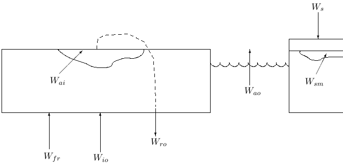

Once the ice tracers are advected, the ice concentration and thickness are timestepped according to the terms on the right:
![{\displaystyle {\begin{aligned}{\frac {DAh_{i}}{Dt}}&={\frac {\rho _{o}}{\rho _{i}}}\left[A(W_{{io}}-W_{{ai}})+(1-A)W_{{ao}}+W_{{fr}}\right]\\{\frac {DA}{Dt}}&={\frac {\rho _{o}}{\rho _{i}h_{i}}}\left[\Phi (1-A)w_{{ao}}+(1-A)W_{{fr}}\right]\;\;\;\;\;0\leq A\leq 1\end{aligned}}}](https://www.myroms.org/myroms.org/v1/media/math/render/svg/0509ede38ba4a6936ecaed513a12a5474c43f7a1)
The term is the "effective thickness", a measure of the ice volume. Its evolution equation is simply quantifying the change in the amount of ice. The ice concentration equation is more interesting in that it provides the partitioning between ice melt/growth on the sides vs. on the top and bottom. The parameter controls this and has differing values for ice melt and retreat. In principle, most of the ice growth is assumed to happen at the base of the ice while rather more of the melt happens on the sides of the ice due to warming of the water in the leads.

The heat fluxes through the ice are based on a simple one layer Semtner (1976) type model with snow on top. The temperature is assumed to be linear within the snow and within the ice. The ice contains brine pockets for a total ice salinity of 3.2 or the surface ocean salinity, whichever is less. The surface ocean temperature and salinity is half a below the surface. The water right below the surface is assumed to be at the freezing temperature; a logarithmic boundary layer is computed having the temperature and salinity matched at freezing.

Similarly, there is a snow equation:
![{\displaystyle {DAh_{s} \over Dt}=\left[A(W_{{s}}-W_{{sm}})\right]}](https://www.myroms.org/myroms.org/v1/media/math/render/svg/f599a128d1f9487891ed37110d3702b6fee7a943)
where and are the snowfall and snow melt rates, respectively, in units of equivalent water. Also in the model is the depth of the melt ponds in spring, which can be up to 0.1 m, after which melting ice contributes to . The melt ponds are not part of the thermal conductivity computations. They could contribute to the albedo computation, but that has been largely commented out.


The ice model thermodynamic variables:
| Name | Description |
|---|---|
| shortwave albedo of water | |
| shortwave albedo of wet ice | |
| shortwave albedo of dry ice | |
| shortwave albedo of wet snow | |
| shortwave albedo of dry snow | |
| snow correction factor | |
| = 2093 J kg K | specific heat of ice |
| = 3990 J kg K | specific heat of water |
| longwave emissivity of water | |
| longwave emissivity of ice | |
| longwave emissivity of snow | |
| enthalpy of the ice/brine system | |
| heat flux from the ocean into the ice | |
| sensible heat | |
| fraction of the solar heating transmitted through a lead into the water below | |
| = 2.04 W m K | thermal conductivity of ice |
| = 0.31 W m K | thermal conductivity of snow |
| = 302 MJ m | latent heat of fusion of ice |
| = 110 MJ m | latent heat of fusion of snow |
| latent heat | |
| incoming longwave radiation | |
| & C/PSU | coefficient in linear equation |
| contribution to equation from freezing water | |
| heat flux out of the snow/ice surface | |
| heat flux out of the ocean surface | |
| heat flux up out of the ice | |
| heat flux up into the ice | |
| heat flux up through the snow | |
| brine fraction in ice | |
| = 910 | density of ice |
| = 3.2 PSU | salinity of the ice |
| incoming shortwave radiation | |
| = W m K | Stefan-Boltzmann constant |
| temperature of the bottom of the ice | |
| temperature of the interior of the ice | |
| temperature at the upper surface of the ice | |
| temperature at the upper surface of the snow | |
| freezing temperature | |
| = | melting temperature of ice |
| = 0 C | melting temperature of snow |
| melt rate on the upper ice/snow surface | |
| freeze rate at the air/water interface | |
| rate of frazil ice growth | |
| freeze rate at the ice/water interface | |
| rate of run-off of surface melt water | |
| snowfall rate | |
| snow melt rate |


The locations of the ice and snow temperatures and the heat fluxes:
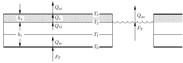

The temperature profile is assumed to be linear between adjacent temperature points. The interior of the ice contains "brine pockets", leading to a prognostic equation for the temperature .
The surface flux to the air is:

The incoming shortwave and longwave radiations are assumed to come from an atmospheric model. The formulae for sensible heat, latent heat, and outgoing longwave radiation are the same as in Parkinson and Washington (1979) and are shown in Radiant Heat Fluxes. The sensible heat is a function of , as is the heat flux through the snow . Setting , we can solve for by setting and linearizing in . As in Parkinson and Washington, if is found to be above the melting temperature, it is set to and the extra energy goes into melting the snow or ice:


![{\displaystyle {\begin{aligned}W_{{ai}}&={\frac {Q_{{ai}}-Q_{{i2}}}{\rho _{o}L_{3}}}\\L_{3}&\equiv \left[E(T_{3},1)-E(T_{1},R_{1})\right]\end{aligned}}}](https://www.myroms.org/myroms.org/v1/media/math/render/svg/01f9457677b087fb5c5d1fa309365dc36ea9dc1e)
Note that plus a small sensible heat correction. We can store water on the surface in melt pools to a fixed depth---everything extra melted at the surface is assumed to flow into the ocean as . The melt ponds however do not contribute to the heat flux computation.

Inside the ice there are brine pockets in which there is salt water at the in situ freezing temperature. It is assumed that the ice has a uniform overall salinity of and that the freezing temperature is a linear function of salinity. The brine fraction is given by

The enthalpy of the combined ice/brine system is given by

Substituting in for and differentiating gives:

Inside the snow, we have

The heat conduction in the upper part of the ice layer is

These can be set equal to each other to solve for

where

Substituting into (\ref{qi2}), we get:


At the bottom of the ice, we have

The difference between and goes into the enthalpy of the ice:


![{\displaystyle \rho _{i}h_{i}\left[{\frac {\partial E}{\partial t}}+{\vec {v}}\cdot \nabla E\right]=Q_{{I0}}-Q_{{I2}}}](https://www.myroms.org/myroms.org/v1/media/math/render/svg/7679952276bf2ae31fd83b0a84231bfb58857d35)
We can use the chain rule to obtain an equation for timestepping :
![{\displaystyle \rho _{i}h_{i}{\frac {\partial E}{\partial T}}\left[{\frac {\partial T_{1}}{\partial t}}+{\vec {v}}\cdot \nabla T_{1}\right]=Q_{{I0}}-Q_{{I2}}}](https://www.myroms.org/myroms.org/v1/media/math/render/svg/4887391f1f0d2bb253c6340baf1e3fc4f5a102a0)
where
![{\displaystyle {\begin{aligned}Q_{{I0}}-Q_{{I2}}&={\frac {2k_{i}}{h_{i}}}\left[(T_{0}-T_{1})-{\frac {(T_{1}-T_{3})}{1+C_{k}}}\right]\\&={\frac {2k_{i}}{h_{i}}}\left[(T_{0}+{\frac {T_{3}-(2+C_{k})T_{1}}{1+C_{k}}}\right]\end{aligned}}}](https://www.myroms.org/myroms.org/v1/media/math/render/svg/4c17baa5f49afea3b1454bfdd40e1cf43620dd04)
Ocean surface boundary conditions
The ocean receives surface stresses from both the atmosphere and the ice, according to the ice concentration:

where the relevant variables are in the following table:
| Variable | Value | Definition |
|---|---|---|
| 3.14 | factor | |
| evaporation | ||
| 0.4 | von Karman's constant | |
| vertical viscosity of seawater | ||
| kinematic viscosity of seawater | ||
| precipitation | ||
| 13.0 | molecular Prandtl number | |
| 0.85 | turbulent Prandtl number | |
| surface salinity | ||
| internal ocean salinity | ||
| 2432 | molecular Schmidt number | |
| stress on the ocean from the ice | ||
| stress on the ocean from the wind | ||
| surface ocean temperature | ||
| internal ocean temperature | ||
| friction velocity | ||
| roughness parameter |


surface salinity () in the presense of ice. We also have and at the uppermost computed ocean point below the surface. In order to solve for and , we assume a Yaglom and Kader, 1974 logarithmic boundary layer. The upper ocean heat flux is:


where

Likewise, we have the following equation for the surface salt flux:

where

The ocean model receives the following heat and salt fluxes:

Mellor and Kantha describe solving simultaneously for the five unknowns , , , and . Instead, we use the old value of to find and therefore . Using the new value of , solve for a new value of and then find the new as the freezing temperature for that salinity:


![{\displaystyle {\begin{aligned}W_{{io}}&={1 \over L_{o}}\left[{Q_{{io}} \over \rho _{o}}+C_{{po}}C_{{T_{z}}}(T_{o}-T)\right]\\S_{0}&={C_{{S_{z}}}S+(W_{{ai}}H(-W_{{ai}})-W_{{io}}))S_{i} \over C_{{S_{z}}}+W_{{ai}}H(-W_{{ai}})+W_{{ro}}-W_{{io}}}\end{aligned}}}](https://www.myroms.org/myroms.org/v1/media/math/render/svg/098eabaf7600f891759e08470f5a2c1e10c546df)
Note that the term is the contribution of melting only, not refreezing of melt ponds.

Frazil ice formation
Following Steele et al. (1989), we check to see if any of the ocean temperatures are below freezing at the end of each timestep. If so, frazil ice is formed, changing the local temperature and salinity. The ice that forms is assumed to instantly float up to the surface and add to the ice layer there. We balance the mass, heat, and salt before and after the ice is formed:

The variables are defined in this table:
| Variable | Value | Definition |
|---|---|---|
| 1994 J kg K | specific heat of ice | |
| 3987 J kg K | specific heat of water | |
| fraction of water that froze | ||
| 3.16e5 J kg | latent heat of fusion | |
| mass of ice formed | ||
| mass of water before freezing | ||
| mass of water after freezing | ||
| constant in freezing equation | ||
| constant in freezing equation | ||
| salinity before freezing | ||
| salinity after freezing | ||
| temperature before freezing | ||
| temperature after freezing |


Defining and dropping terms of order
leads to:


![{\displaystyle T_{2}=T_{1}+\gamma \left[{\frac {L}{C_{{pw}}}}+T_{1}\left(1-{\frac {C_{{pi}}}{C_{{pw}}}}\right)\right]}](https://www.myroms.org/myroms.org/v1/media/math/render/svg/079b5f619051b0584bfbe8a2bba5b8475a3bc2c6)

We also want the final temperature and salinity to be on the freezing line, which we approximate as:

We can then solve for :

The ocean is checked at each depth and at each timestep for supercooling. If the water is below freezing, the temperature and salinity are adjusted as in equations (\ref{t2eq}) and (\ref{s2eq}) and the ice above is thickened by the amount:
