Difference between revisions of "Nested Grids"
| Line 111: | Line 111: | ||
Notice the '''duality''' of a ROMS nested grid: data '''donor''' in one '''contact region''' and data '''receiver''' in its conjugate '''contact region'''. The exchange of information is always two-way. This explains why we prefer to use the '''donor''' and '''receiver''' categories instead of the usual '''parent''' and '''child''' descriptions found in the literature. | Notice the '''duality''' of a ROMS nested grid: data '''donor''' in one '''contact region''' and data '''receiver''' in its conjugate '''contact region'''. The exchange of information is always two-way. This explains why we prefer to use the '''donor''' and '''receiver''' categories instead of the usual '''parent''' and '''child''' descriptions found in the literature. | ||
The contact points are processed outside of ROMS and all the connectivity within nested grids is read from an input NetCDF file. This facilitates the configuration of various grid Sub-Classes. It simplifies tremendously the processing of such points in parallel computations. It also give the user a full editing control of the contact points. The contact points | The contact points are processed outside of ROMS and all the connectivity within nested grids is read from an input NetCDF file. This facilitates the configuration of various grid Sub-Classes. It simplifies tremendously the processing of such points in parallel computations. It also give the user a full editing control of the contact points. The contact points need to be set-up once for a particular application. | ||
In ROMS, the contact region and contact point are managed with the following Fortran-90 structure in [[Modules#mod_nesting.F|mod_nesting.F]]: | In ROMS, the contact region and contact point are managed with the following Fortran-90 structure in [[Modules#mod_nesting.F|mod_nesting.F]]: | ||
| Line 314: | Line 314: | ||
:history = "Contact points created by contact.m and written by write_contact.m" ; </span> | :history = "Contact points created by contact.m and written by write_contact.m" ; </span> | ||
Notice that the variable dimensions (<span class="red">Hweight</span>) are in '''row-major''' order since this is the output from '''ncdump'''. However, the data is stored in '''column-major''' order because this file will be processed by ROMS in Fortran-90. The strategy here is to '''pack''' the contact points information for each contact region in a long vector. Several indices are available to '''unpack''' the data into the Fortran-90 contact structures for ρ-, u-, and v-points. Although NetCDF-4 supports derived type structures via the HDF5 library, a simpler Metadata model is chosen for interoperability. Notice that the contact points NetCDF file contains also the values for the various grid metrics needed in ROMS numerical kernel. Only the horizontal interpolation weights are provided here since they are always the same for a particular configuration. The vertical interpolation weights are computed internally in ROMS at each time step because of the time dependency of the vertical coordinates to the evolution of the free-surface. | Notice that the variable dimensions (<span class="red">Hweight</span>) are in '''row-major''' order since this is the output from '''ncdump'''. However, the data is stored in '''column-major''' order because this file will be processed by ROMS in Fortran-90. The strategy here is to '''pack''' the contact points information for each contact region in a long vector. Several indices are available to '''unpack''' the data into the Fortran-90 contact structures for '''&rho''';-, '''u'''-, and '''v'''-points. Although '''NetCDF-4''' supports derived type structures via the '''HDF5''' library, a simpler Metadata model is chosen for interoperability. Notice that the contact points NetCDF file contains also the values for the various grid metrics needed in ROMS numerical kernel. Only the horizontal interpolation weights are provided here since they are always the same for a particular configuration. The vertical interpolation weights are computed internally in ROMS at each time step because of the time dependency of the vertical coordinates to the evolution of the free-surface. | ||
</wikitex> | </wikitex> | ||
Revision as of 13:54, 25 April 2012
| Nested Grids Menu | |
|---|---|
| 1. Introduction | |
| 2. Matlab Processing Scripts |
Introduction
ROMS has a nested design structure for the temporal coupling between a hierarchy of donor and receiver grids. All the state model variables are dynamically allocated and passed as arguments to the computational routines via Fortran-90 dereferenced pointer structures. All private arrays are automatic; their size is determined when the procedure is entered. This code structure facilitates computations over nested grids of different topologies. There are three types of nesting capabilities in ROMS:
- Mosaics Grids which connect several grids along their edges,
- Composite Grids which allow overlap regions of aligned and non-aligned grids, and
- Refinement Grids which provide increased resolution (3:1, 5:1, or 7:1) in a specific region.
The mosaic and composite grid code infrastructures are identical. The differences are geometrical and primary based on the alignment between adjacent grids. All the mosaic grids are exactly aligned with the adjacent grid. In general, the mosaic grids are special case of the composite grids.
The nested grid implementation was divided in three sequential phases:
- Phase I, released on April 2011 as ROMS version 3.5, included major updates to the nonlinear (NLM), perturbation tangent linear (TLM), finite-amplitude tangent linear (RPM), and adjoint (ADM) models numerical kernels to allow different horizontal I- and J-ranges in the DO-loops to permit operations on various nested grid classes (refinement, mosaics, and composite) and nesting layers (refinement and composite grid combinations). This facilitates the computation of any horizontal operator (advection, diffusion, gradient, etc.) in the nesting contact regions and avoids the need for cumbersome lateral boundary conditions on the model variables and their associated flux/gradient values. The advantage of this approach is that it is generic to any discrete horizontal operator. The contact region is an extended section of the grid that overlays an adjacent grid. The strategy is to compute the full horizontal operator at the contact points between nested grids instead of specifying boundary conditions.
- Phase II, released on September 2011 as ROMS version 3.6, included a major overhaul of lateral boundary conditions. All their associated C-preprocessing options were eliminated and replaced with logical switches that depend on the nested grid, if any. This facilitates, in a generic way, the processing or not of lateral boundary conditions in applications with nested grids. In nesting applications, the values at the lateral boundary points are computed directly in the contact region by the numerical kernel. Partial lateral boundary conditions are allowed by combining specified conditions (like closed, gradient, and others) with nested contact points. In addition, the logical switches allow different lateral boundary conditions types between active (temperature and salinity) and passive (biology, sediment, inert, etc.) tracers. The lateral boundary condition switches for each state variable and boundary edge are now specified in ROMS input script file, ocean.in.
- Phase III, to be released soon as ROMS version 3.7, includes the nesting calls to ROMS main time-stepping routines, main2d and main3d. The routine main2d is only used in shallow-water 2D barotropic applications whereas main3d is used in full 3D baroclinic applications. Several new routines will be added to process the information that it is required in the contact region, what information needs to be exchanged from/to another grid, and when to exchange it.
In grid refinement applications, the information is exchanged at the begginning of the full time-step (top of main2d or main3d). Contrarily, in composite grids applications, the information is exchanged between each sub-time step call in main2d or main3d. That is, the composite donor and receiver grids need to sub-time step the 2D momentum equations before any of them start solving and coupling the 3D momentum equations. Therefore, the governing equations are solved and nested in a synchronous fashion. The concept of nesting layers is introduced to allow applications with both composite grids and refinement grid combinations, as shown in the diagram below for the Refinement and Partial Boundary Composite Sub-Class. Here, two nesting layers are required. In the first nesting layer, the composite grids 1 and 2 are synchronously sub-time stepped for each governing equation term. Then, in the second and last nesting layer, the refinement grid 3 is time stepped and the information between donor (1) and receiver refinement (3) grids are exchanged at the beginning of the time step for both contact regions: coarse-to-fine and fine-to-coarse. The exchange between grids is two-way.
The current plan is to move to ROMS version 4.0 when all complex new developments are fully stable and tested. The design and implementation is fully adjointable and we have big plans in the future to support the adjoint-based algorithms, like 4D-Var, over selected or all nested grids.
Nested Grids Classes
<wikitex> The ROMS nested grid design includes three Super-Classes and several Sub-Classes:
- Composite Grids Super-Class:
- Mosaic Grids Sub-Class
- Composite Overlap Grids Sub-Class
- Partial Boundary Composite Grids Sub-Class
- Complex Estuary Composite Grids Sub-Class
- Refinement Grids Super-Class:
- Single Refinement Sub-Class
- Multiple Refinement Sub-Class
- Composite and Refinement Combination Super-Class:
- Refinement and Partial Boundary Composite Sub-Class
- Complex Estuary Refinement-Composite Sub-Class
Hence, there are several possibilities and combinations. The design is flexible enough to allow complex nested grid configurations in coastal applications. These capabilities are better illustrated with diagrams of the different Sub-Classes. The diagrams are all in terms of computational coordinates ($\xi$, $\eta$) or fractional ($i$, $j$) coordinates. Therefore we have squares and rectangles that may map to physical curvilinear coordinates.
- Composite Grids
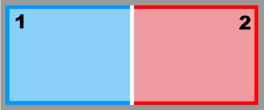
Mosaic Sub-Class:
Ngrids = 2
NestLayers = 1
GridsInLayer = 1
Ncontact = 2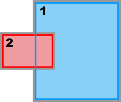
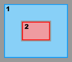
Composite Overlap Sub-Class:
Ngrids = 2
NestLayers = 1
GridsInLayer = 1
Ncontact = 2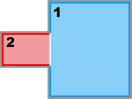
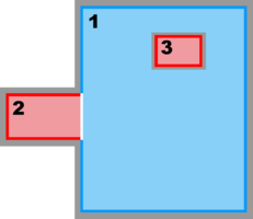
Partial Boundary Composite Sub-Class:
Ngrids = 2
NestLayers = 1
GridsInLayer = 1
Ncontact = 2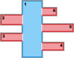
Complex Estuary Composite Sub-Class:
Ngrids = 6
NestLayers = 1
GridsInLayer = 6
Ncontact = 10


- Refinement Grids
Single Refinement Sub-Class:
Ngrids = 2
NestLayers = 2
GridsInLayer = 1 1
Ncontact = 2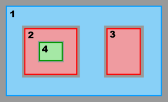
Multiple Refinement Sub-Class:
Ngrids = 4
NestLayers = 3
GridsInLayer = 1 2 1
Ncontact = 6


- Composite and Refinement Combination Grids
Refinement and Partial Boundary Composite Sub-Class:
Ngrids = 3
NestLayers = 2
GridsInLayer = 2 1
Ncontact = 4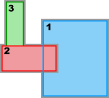
Complex Estuary Refinement-Composite Sub-Class:
Ngrids = 3
NestLayers = 2
GridsInLayer = 1 2
Ncontact = 4


![]() Warning 1: The order of nested grids in ROMS is extremely important. We need to follow such order when specifying parameters in all ROMS standard input scripts: ocean.in, biology.in, sediment.in, and so on. The numeric order is shown above for all nested grid Sub-Classes. It depends on a particular configuration topology, number of nested layers, and on the physical circulation. Generally, the larger/coarser grid is first in the order list. Therefore, users need to order their grids wisely...
Warning 1: The order of nested grids in ROMS is extremely important. We need to follow such order when specifying parameters in all ROMS standard input scripts: ocean.in, biology.in, sediment.in, and so on. The numeric order is shown above for all nested grid Sub-Classes. It depends on a particular configuration topology, number of nested layers, and on the physical circulation. Generally, the larger/coarser grid is first in the order list. Therefore, users need to order their grids wisely...
![]() Warning 2: In composite grids, it is assumed that the donor and the receiver grids have the same time-step size. This is done to avoid the time interpolation between donor and receiver grids. Only spatial interpolations are possible and carried out. This is due to the fact that composite grids need to solve the governing equations in a synchronous fashion, as explained in above. In refinement grids, it is assumed that the donor and receiver grids are an integer factor (RefineScale) of the grid-size and time-step size. Therefore, time interpolation and time integration is possible between donor and receiver grids.
Warning 2: In composite grids, it is assumed that the donor and the receiver grids have the same time-step size. This is done to avoid the time interpolation between donor and receiver grids. Only spatial interpolations are possible and carried out. This is due to the fact that composite grids need to solve the governing equations in a synchronous fashion, as explained in above. In refinement grids, it is assumed that the donor and receiver grids are an integer factor (RefineScale) of the grid-size and time-step size. Therefore, time interpolation and time integration is possible between donor and receiver grids.
![]() Warning 3: In refinement grid applications, we do not recommend to use refinement factors exceeding the 1:7 ratio. Mostly everybody consider either the 1:3 or 1:5 ratio between donor and receiver refinement grid applications. Notice that the refinement factor (RefineScale) in C-grids needs to have an integer value given by 2n + 1 for n=1,2,3,... to guarantee always a ρ-point at the center of the grid cell.
Warning 3: In refinement grid applications, we do not recommend to use refinement factors exceeding the 1:7 ratio. Mostly everybody consider either the 1:3 or 1:5 ratio between donor and receiver refinement grid applications. Notice that the refinement factor (RefineScale) in C-grids needs to have an integer value given by 2n + 1 for n=1,2,3,... to guarantee always a ρ-point at the center of the grid cell.
![]() Usually, finer resolution is required to resolve estuary regions or other coastal features in a particular application. In this case, we should consider a refinement grid with Land/Sea masking in such areas. This case is illustrated in the Complex Estuary Refinement-Composite Sub-Class diagram above. Notice that the refinement grid 2 has an adjacent composite grid 3 of similar spatial resolution, so all the grids in the second nested layer have the same time step. As you can see, ROMS nesting capabilities are powerful but it requires knowledge and expertise. We highly recommend users to acquire this knowledge before configure their own nested grid applications. This knowledge is difficult to explain in words, but easier to show with the diagrams in this page. We need to gain experience with this capability.
Usually, finer resolution is required to resolve estuary regions or other coastal features in a particular application. In this case, we should consider a refinement grid with Land/Sea masking in such areas. This case is illustrated in the Complex Estuary Refinement-Composite Sub-Class diagram above. Notice that the refinement grid 2 has an adjacent composite grid 3 of similar spatial resolution, so all the grids in the second nested layer have the same time step. As you can see, ROMS nesting capabilities are powerful but it requires knowledge and expertise. We highly recommend users to acquire this knowledge before configure their own nested grid applications. This knowledge is difficult to explain in words, but easier to show with the diagrams in this page. We need to gain experience with this capability.
</wikitex>
Contact Regions and Contact Points
<wikitex> A contact region is an extended section of the grid that overlays or is adjacent to a nested grid. A contact point is a grid cell inside the contact region. The contact points are located according to the staggered Arakawa C-grid horizontal positions. Therefore, we have contact points at the ρ-, ψ-, u-, and v-points. However, the ψ-points are only used to define the physical grid perimeters within a contact region. ROMS does not have state variables located at ψ-points; vorticity is not explicitly specified in the governing equations. In a nested application, there are (Ngrids-1)*2 contact regions. Each contact region has a receiver grid and donor grid. The contact points of the receiver grid are processed using the donor grid cell containing the contact point. The contact points are coincident if the receiver and donor grids occupy the same position, p = q = 0 in diagram below. If coincident grids, the receiver grid contact point data is just filled using the donor data. Otherwise, if not coincident, the receiver grid data is linearly interpolated from the donor grid cell containing the contact point.


Here, the suffixes dg and rg are for the donor grid and receiver grid, respectively. The horizontal interpolation weights are as follows:
- Hweight(1,:) = (1.0 - p) * (1.0 - q)
- Hweight(2,:) = p * (1.0 - q)
- Hweight(3,:) = p * q
- Hweight(4,:) = (1.0 - p) * q
These horizontal interpolation weights are computed outside ROMS and read from contact points NetCDF file. Then, the contact point for a 2D state variable in the receiver grid is computed from the donor grid as:
- V(Irg, Jrg) = Hweight(1,:) * F2D(Idg, Jdg) +
- Hweight(2,:) * F2D(Idg+1, Jdg) +
- Hweight(3,:) * F2D(Idg+1, Jdg+1) +
- Hweight(4,:) * F2D(Idg, Jdg+1)
- V(Irg, Jrg) = Hweight(1,:) * F2D(Idg, Jdg) +
If coincident contact points between data donor and data receiver grids, p = q = 0,
- Hweight(1,:) = 1.0
- Hweight(2,:) = 0.0
- Hweight(3,:) = 0.0
- Hweight(4,:) = 0.0
and
- V(Irg, Jrg) = Hweight(1,:) * F2D(Idg, Jdg)
Notice the duality of a ROMS nested grid: data donor in one contact region and data receiver in its conjugate contact region. The exchange of information is always two-way. This explains why we prefer to use the donor and receiver categories instead of the usual parent and child descriptions found in the literature.
The contact points are processed outside of ROMS and all the connectivity within nested grids is read from an input NetCDF file. This facilitates the configuration of various grid Sub-Classes. It simplifies tremendously the processing of such points in parallel computations. It also give the user a full editing control of the contact points. The contact points need to be set-up once for a particular application.
In ROMS, the contact region and contact point are managed with the following Fortran-90 structure in mod_nesting.F:
     integer :: Ncontact                             ! total number of contact regions

     TYPE T_NGC

       logical :: coincident                         ! coincident donor/receiver grid switch, p=q=0
       logical :: interpolate                        ! switch to perform vertical interpolation

       integer :: donor_grid                         ! data donor grid number
       integer :: receiver_grid                      ! data receiver grid number

       integer :: Npoints                            ! number of points in contact region

       integer, pointer :: Irg(:)                    ! receiver grid, I-contact point
       integer, pointer :: Jrg(:)                    ! receiver grid, J-contact point

       integer, pointer :: Idg(:)                    ! donor grid, contact cell I-left   index
       integer, pointer :: Jdg(:)                    ! donor grid, contact cell J-bottom index
       integer, pointer :: Kdg(:,:)                  ! donor grid, contact cell K-index

       real(r8), pointer :: Hweight(:,:)             ! horizontal interpolation weights
       real(r8), pointer :: Vweight(:,:,:)           ! vertical   interpolation weights

     END TYPE T_NGC

     TYPE (T_NGC), allocatable :: Rcontact(:)        ! contact points at RHO-points, [Ncontact]
     TYPE (T_NGC), allocatable :: Ucontact(:)        ! contact points at U-points,   [Ncontact]
     TYPE (T_NGC), allocatable :: Vcontact(:)        ! contact points at V-points,   [Ncontact]
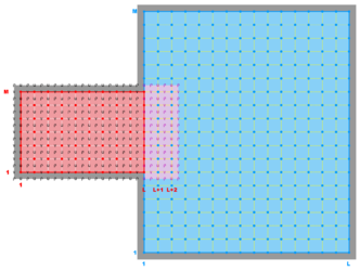
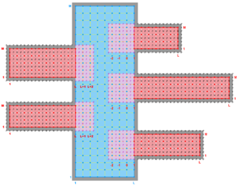
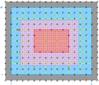
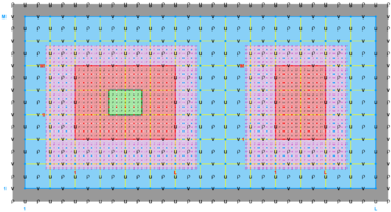
The diagrams below show the contact regions and contact points for each nesting Sub-Class. Each diagram shows the contact region and its contact points colored purple as a transition between the blue and red grids. Color is used to illustrate the nesting role between donor and receiver grids. It also shows the number of nesting layers (NestLayer) and number grids in each nested layer (GridsInLayer). Notice that there is an extra contact point to the left and bottom of the nested grid. This is due to ROMS index enumeration system for staggered, Arakawa C-grids. A left-bottom enumeration system is used: the i-index for u-points to the left of the ρ-point have the same value; the j-index for v-points to the bottom of the ρ-point have the same value.
- Mosaic Sub-Class
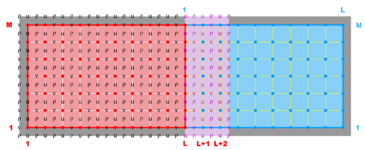
Ngrids = 2
NestLayers = 1
GridsInLayer = 2
Ncontact = 2
Donor Grid = blue
Receiver Grid = red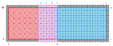
Ngrids = 2
NestLayers = 1
GridsInLayer = 2
Ncontact = 2
Donor Grid = red
Receiver Grid = blue


- Composite Overlap Sub-Class
Ngrids = 2
NestLayers = 1
GridsInLayer = 2
Ncontact = 2
Donor Grid = blue
Receiver Grid = red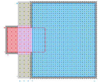
Ngrids = 2
NestLayers = 1
GridsInLayer = 2
Ncontact = 2
Donor Grid = red
Receiver Grid = blue


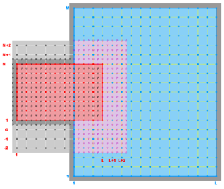
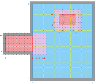
- Partial Boundary Composite Sub-Class
Ngrids = 2
NestLayers = 1
GridsInLayer = 2
Ncontact = 2
Donor Grid = blue
Receiver Grid = red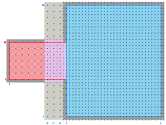
Ngrids = 2
NestLayers = 1
GridsInLayer = 2
Ncontact = 2
Donor Grid = red
Receiver Grid = blue


- Complex Estuary Composite Sub-Class
Ngrids = 2
NestLayers = 1
GridsInLayer = 2
Ncontact = 2
Donor Grid = blue
Receiver Grid = red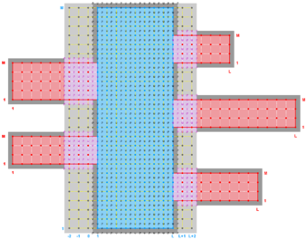
Ngrids = 2
NestLayers = 1
GridsInLayer = 2
Ncontact = 2
Donor Grid = red
Receiver Grid = blue


- Single Refinement Sub-Class
Ngrids = 2
NestLayers = 2
GridsInLayer = 1 1
Ncontact = 2
Donor Grid = blue
Receiver Grid = red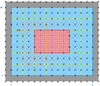
Ngrids = 2
NestLayers = 2
GridsInLayer = 1 1
Ncontact = 2
Donor Grid = red
Receiver Grid = blue


- Multiple Refinement Sub-Class
Ngrids = 4
NestLayers = 3
GridsInLayer = 1 2 1
Ncontact = 6
Donor Grid = blue
Receiver Grid = red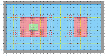
Ngrids = 4
NestLayers = 3
GridsInLayer = 1 2 1
Ncontact = 6
Donor Grid = red
Receiver Grid = blue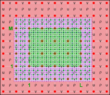
Ngrids = 4
NestLayers = 3
GridsInLayer = 1 2 1
Ncontact = 6
Donor Grid = red
Receiver Grid = green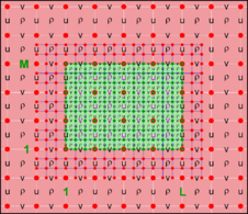
Ngrids = 4
NestLayers = 3
GridsInLayer = 1 2 1
Ncontact = 6
Donor Grid = green
Receiver Grid = red


- Refinement & Partial Boundary Composite Sub-Class
Ngrids = 3
NestLayers = 2
GridsInLayer = 2 1
Ncontact = 4
Donor Grid = blue
Receiver Grid = red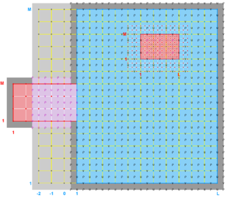
Ngrids = 3
NestLayers = 2
GridsInLayer = 2 1
Ncontact = 4
Donor Grid = red
Receiver Grid = blue


</wikitex>
Metadata
<wikitex> The contact regions and contact points are processed outside ROMS and read in from a NetCDF file with the following Metadata structure:
  dimensions:

       Ngrids = 2 ;
       Ncontact = 2 ;
       Nweights = 4 ;
       datum = 98 ;

  variables:

       int spherical ;
               spherical:long_name = "grid type logical switch" ;
               spherical:flag_values = 0, 1 ;
               spherical:flag_meanings = "Cartesian spherical" ;
       int Lm(Ngrids) ;
               Lm:long_name = "number of interior RHO-points in the I-direction" ;
       int Mm(Ngrids) ;
               Mm:long_name = "number of interior RHO-points in the J-direction" ;
       int coincident(Ngrids) ;
               coincident:long_name = "coincident donor and receiver grids logical switch" ;
               coincident:flag_values = 0, 1 ;
               coincident:flag_meanings = "false true" ;
       int composite(Ngrids) ;
               composite:long_name = "composite grid type logical switch" ;
               composite:flag_values = 0, 1 ;
               composite:flag_meanings = "false true" ;
       int mosaic(Ngrids) ;
               mosaic:long_name = "mosaic grid type logical switch" ;
               mosaic:flag_values = 0, 1 ;
               mosaic:flag_meanings = "false true" ;
       int refinement(Ngrids) ;
               refinement:long_name = "refinement grid type logical switch" ;
               refinement:flag_values = 0, 1 ;
               refinement:flag_meanings = "false true" ;
       int refine_factor(Ngrids) ;
               refine_factor:long_name = "refinement factor from donor grid" ;
       int interpolate(Ncontact) ;
               interpolate:long_name = "vertical interpolation at contact points logical switch" ;
               interpolate:flag_values = 0, 1 ;
               interpolate:flag_meanings = "false true" ;
       int donor_grid(Ncontact) ;
               donor_grid:long_name = "data donor grid number" ;
       int receiver_grid(Ncontact) ;
               receiver_grid:long_name = "data receiver grid number" ;
       int NstrR(Ncontact) ;
               NstrR:long_name = "starting contact RHO-point index in data vector" ;
       int NendR(Ncontact) ;
               NendR:long_name = "ending contact RHO-point index in data vector" ;
       int NstrU(Ncontact) ;
               NstrU:long_name = "starting contact U-point index in data vector" ;
       int NendU(Ncontact) ;
               NendU:long_name = "ending contact U-point index in data vector" ;
       int NstrV(Ncontact) ;
               NstrV:long_name = "starting contact V-point index in data vector" ;
       int NendV(Ncontact) ;
               NendV:long_name = "ending contact V-point index in data vector" ;
       int contact_region(datum) ;
               contact_region:long_name = "contact region number" ;
       int on_boundary(datum) ;
               on_boundary:long_name = "contact point on receiver grid physical boundary" ;
               on_boundary:flag_values = 0, 1, 2, 3, 4 ;
               on_boundary:flag_meanings = "false western southern eastern northern" ;
       int Idg(datum) ;
               Idg:long_name = "I-left index of donor cell containing contact point" ;
       int Jdg(datum) ;
               Jdg:long_name = "J-bottom index of donor cell containing contact point" ;
       int Irg(datum) ;
               Irg:long_name = "receiver grid I-index of contact point" ;
               Irg:coordinates = "Xrg Yrg" ;
       int Jrg(datum) ;
               Jrg:long_name = "receiver grid J-index of contact point" ;
               Jrg:coordinates = "Xrg Yrg" ;
       double Xrg(datum) ;
               Xrg:long_name = "X-location of receiver grid contact points" ;
               Xrg:units = "meter" ;
       double Yrg(datum) ;
               Yrg:long_name = "Y-location of receiver grid contact points" ;
               Yrg:units = "meter" ;
       double Hweight(datum, Nweights) ;
               Hweight:long_name = "horizontal interpolation weights" ;
               Hweight:coordinates = "Xrg Yrg" ;
       double h(datum) ;
               h:long_name = "bathymetry at RHO-points" ;
               h:units = "meter" ;
               h:coordinates = "Xrg Yrg" ;
               h:_FillValue = 1.e+37 ;
       double f(datum) ;
               f:long_name = "Coriolis parameter at RHO-points" ;
               f:units = "second-1" ;
               f:coordinates = "Xrg Yrg" ;
               f:_FillValue = 1.e+37 ;
       double pm(datum) ;
               pm:long_name = "curvilinear coordinate metric in XI" ;
               pm:units = "meter-1" ;
               pm:coordinates = "Xrg Yrg" ;
               pm:_FillValue = 1.e+37 ;
       double pn(datum) ;
               pn:long_name = "curvilinear coordinate metric in ETA" ;
               pn:units = "meter-1" ;
               pn:coordinates = "Xrg Yrg" ;
               pn:_FillValue = 1.e+37 ;
       double dndx(datum) ;
               dndx:long_name = "XI-derivative of inverse metric factor pn" ;
               dndx:units = "meter" ;
               dndx:coordinates = "Xrg Yrg" ;
               dndx:_FillValue = 1.e+37 ;
       double dmde(datum) ;
               dmde:long_name = "ETA-derivative of inverse metric factor pm" ;
               dmde:units = "meter" ;
               dmde:coordinates = "Xrg Yrg" ;
               dmde:_FillValue = 1.e+37 ;
       double angle(datum) ;
               angle:long_name = "angle between XI-axis and EAST" ;
               angle:units = "radians" ;
               angle:coordinates = "Xrg Yrg" ;
               angle:_FillValue = 1.e+37 ;
       double mask(datum) ;
               mask:long_name = "land-sea mask of contact points" ;
               mask:flag_values = 0., 1. ;
               mask:flag_meanings = "land water" ;
               mask:coordinates = "Xrg Yrg" ;

  global attributes:

               :type = "ROMS Nesting Contact Regions Data" ;
               :grid_files = " \n",
                       "/Users/arango/ocean/repository/TestCases/dogbone/Data/dogbone_grd_left.nc \n",
                       "/Users/arango/ocean/repository/TestCases/dogbone/Data/dogbone_grd_right.nc" ;
               :history = "Contact points created by contact.m and written by write_contact.m" ;
Notice that the variable dimensions (Hweight) are in row-major order since this is the output from ncdump. However, the data is stored in column-major order because this file will be processed by ROMS in Fortran-90. The strategy here is to pack the contact points information for each contact region in a long vector. Several indices are available to unpack the data into the Fortran-90 contact structures for ρ-, u-, and v-points. Although NetCDF-4 supports derived type structures via the HDF5 library, a simpler Metadata model is chosen for interoperability. Notice that the contact points NetCDF file contains also the values for the various grid metrics needed in ROMS numerical kernel. Only the horizontal interpolation weights are provided here since they are always the same for a particular configuration. The vertical interpolation weights are computed internally in ROMS at each time step because of the time dependency of the vertical coordinates to the evolution of the free-surface.
</wikitex>