Difference between revisions of "INLET TEST CASE"
| (32 intermediate revisions by 4 users not shown) | |||
| Line 1: | Line 1: | ||
<div class="title">Inlet Test Case</div> | <div class="title">Inlet Test Case</div> | ||
'''Input Files:''' [[media:Inlet_test_config.zip| zip file with complete inputs ]], tested with ROMS SVN version 291. | |||
'''Output Files:''' [[media:INLET_TEST_SVN_R291_Ocean_his.nc | history file (ocean_his.nc) ]], produced by ROMS SVN version 291. | |||
This test case couples ROMS and [[SWAN]] directly using the Modeling Coupling Toolkit (MCT) library. To run this application the user needs to activate [[Options#INLET_TEST|INLET_TEST]]. It only can be run in distributed-memory (MPI) since the parallel threads are split to run both ROMS and SWAN at the same time. This test illustrates the | |||
significance of wave-current coupling. This application and coupling methodology is described in [[Bibliography#WarnerJC_2008a|Warner ''et al.'' (2008)]]. | |||
( | This test case models and idealized tidal inlet system. The model domain is a 15x14 km rectangle with a uniform initial depth of 4 m. The model setup parameters are shown in the table below. The domain is separated into two regions: the seaward (top) and back-barrier (bottom) regions. The seaward region is open with radiation conditions on the western, northern and eastern edges. The back-barrier region is enclosed with four walls and is connected to the seaward region through a 2 km wide inlet. The model is forced by a tide and waves. An oscillating water level is imposed on the northern edge with a tidal amplitude of 1 m. Waves are also imposed on the northern edge with a height of 1 m, directed to the south with a period of 10s. | ||
Table 1. Important model parameters: | |||
{| border="1" cellspacing="0" cellpadding="5" align="center" | |||
!Model Parameter | |||
!Variable | |||
!Value | |||
|- | |||
|length, width, depth | |||
|[[Variables#Xsize|Xsize]], [[Variables#Esize|Esize]], [[Variables#hmax|hmax]] | |||
|15000 m, 14000 m, 4.0 m | |||
|- | |||
|number of grid spacings | |||
|[[Variables#Lm|Lm]], [[Variables#Mm|Mm]], [[Variables#N|N]] | |||
|75, 70, 10 | |||
|- | |||
|bottom Roughness | |||
|[[Variables#Zob|Zob]] | |||
|0.015 m | |||
|- | |||
|time step | |||
|[[Variables#dt|dt]] | |||
|10 s | |||
|- | |||
|simulation steps | |||
|[[Variables#ntimes|ntimes]] | |||
|17280 steps (2 days) | |||
|- | |||
|morphology factor | |||
|[[Variables#morph_fac|morph_fac]] | |||
|10 (=20 day scaled simulation) | |||
|- | |||
|grain size | |||
|[[Variables#Sd50|Sd50]] | |||
|0.10 mm | |||
|- | |||
|settle velocity | |||
|[[Variables#Wsed|Wsed]] | |||
|11.0 mm s<sup>-1</sup> | |||
|- | |||
|erosion rate | |||
|[[Variables#Erate|Erate]] | |||
|5 x 10<sup>-3</sup> kg m<sup>-2</sup>s<sup>-1</sup> | |||
|- | |||
|critical stress | |||
|[[Variables#tau_cd|tau_cd]], [[Variables#tau_ce|tau_ce]] | |||
|0.10 Nm<sup>-2</sup> | |||
|- | |||
|porosity | |||
|[[Variables#poros|poros]] | |||
|0.50 | |||
|- | |||
|bed thickness | |||
|[[Variables#bed|bed(:, :, :, ithck)]] | |||
|10.0 m | |||
|- | |||
|northern edge tide | |||
|A, T<sub>t</sub> | |||
|1.0 m, 12 h | |||
|- | |||
|northern edge wave height | |||
|H<sub>sig</sub> | |||
|2 m | |||
|- | |||
|northern edge wave period | |||
|T | |||
|10 s | |||
|- | |||
|northern edge wave direction | |||
|θ | |||
|from 0° (from North) | |||
|- | |||
|} | |||
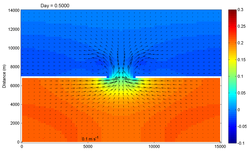
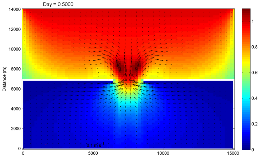
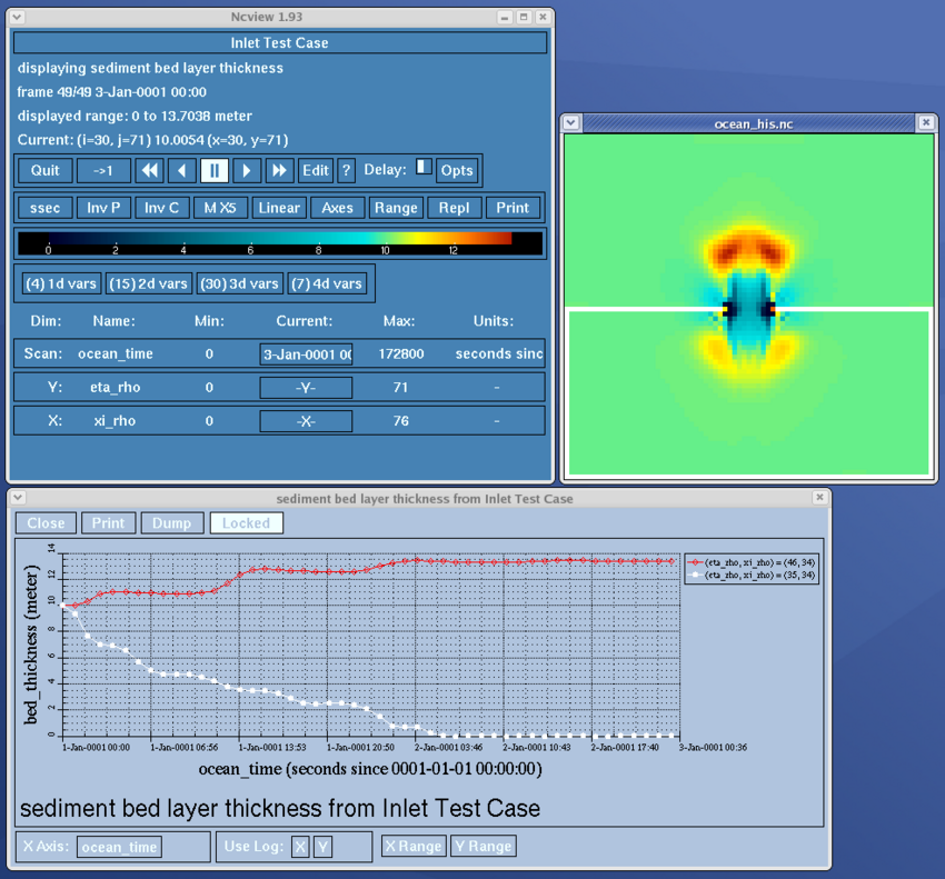
Below we provide a brief example of the model output. | |||
[[Image:Inlet_test_zeta_day0.5.png|thumb|850px|none|<center><b>Figure 1:</b> ROMS output of free surface and barotropic currents at t=0.5 days.</center>]] | |||
[[Image:Inlet_test_Hwave_day0.5.png|thumb|850px|none|<center><b>Figure 2:</b> SWAN output of wave height (Hwave, m) and barotropic currents.</center>]] | |||
[[Image:Inlet_test_final_bed.png|thumb|850px|none|<center><b>Figure 3:</b> Final bed_thickness after 2.0 days. Time series are from locations of maximum erosion and deposition.</center>]] | |||
Latest revision as of 16:56, 9 January 2009
Input Files: zip file with complete inputs , tested with ROMS SVN version 291.
Output Files: history file (ocean_his.nc) , produced by ROMS SVN version 291.
This test case couples ROMS and SWAN directly using the Modeling Coupling Toolkit (MCT) library. To run this application the user needs to activate INLET_TEST. It only can be run in distributed-memory (MPI) since the parallel threads are split to run both ROMS and SWAN at the same time. This test illustrates the
significance of wave-current coupling. This application and coupling methodology is described in Warner et al. (2008).
This test case models and idealized tidal inlet system. The model domain is a 15x14 km rectangle with a uniform initial depth of 4 m. The model setup parameters are shown in the table below. The domain is separated into two regions: the seaward (top) and back-barrier (bottom) regions. The seaward region is open with radiation conditions on the western, northern and eastern edges. The back-barrier region is enclosed with four walls and is connected to the seaward region through a 2 km wide inlet. The model is forced by a tide and waves. An oscillating water level is imposed on the northern edge with a tidal amplitude of 1 m. Waves are also imposed on the northern edge with a height of 1 m, directed to the south with a period of 10s.
Table 1. Important model parameters:
| Model Parameter | Variable | Value |
|---|---|---|
| length, width, depth | Xsize, Esize, hmax | 15000 m, 14000 m, 4.0 m |
| number of grid spacings | Lm, Mm, N | 75, 70, 10 |
| bottom Roughness | Zob | 0.015 m |
| time step | dt | 10 s |
| simulation steps | ntimes | 17280 steps (2 days) |
| morphology factor | morph_fac | 10 (=20 day scaled simulation) |
| grain size | Sd50 | 0.10 mm |
| settle velocity | Wsed | 11.0 mm s-1 |
| erosion rate | Erate | 5 x 10⁻³ kg m-2s-1 |
| critical stress | tau_cd, tau_ce | 0.10 Nm-2 |
| porosity | poros | 0.50 |
| bed thickness | bed(:, :, :, ithck) | 10.0 m |
| northern edge tide | A, Tt | 1.0 m, 12 h |
| northern edge wave height | Hsig | 2 m |
| northern edge wave period | T | 10 s |
| northern edge wave direction | θ | from 0° (from North) |
Below we provide a brief example of the model output.


