I4DVAR

Incremental 4D Variational Data Assimilation

This memo describes a series of calculations using the new preconditioned version of the ROMS I4DVAR algorithm based on the Lanczos algorithm. This driver in ROMS is referred to as cgradient_lanczos.h and will become the default and only I4DVAR option that will be available and maintained for ROMS.

The conjugate gradient solver for ROMS I4DVAR is based on the Lanczos method as described by Fisher (1997, 1998). Two versions of preconditioning are available in ROMS I4DVAR: these are "spectral" preconditioning as described by Fisher (1998), and "Ritz" preconditioning as described by Tshimanga et al. (2008). The "spectral" and "Ritz" nomenclature used here follows that adopted by Tshimanga et al. (2008). The actual implementation of both preconditioners is based on the PhD thesis of Tshimanga (2007).

The model configuration used in all of the following experiments is the Intra-Americas Sea with $40~{\rm {km}}$ resolution. Details of the model set-up, forcing, boundary conditions, and I4DVAR configuration are described in Powell et al. (2008). The multivariate balance operator is not used in any of these calculations, and only the initial conditions are adjusted. Familiarity with I4DVAR and its implementation in ROMS is assumed.

The Preconditioners

Following Tshimanga et al. (2008) the cost function can be expressed in incremental form as:

$$J(\delta {\bf {x}}^{k})={\frac {1}{2}}(\delta {\bf {x}}^{k}-{\bf {d}}_{b}^{k-1})^{T}{\bf {B}}^{-1}(\delta {\bf {x}}^{k}-{\bf {d}}_{b}^{k-1})+{\frac {1}{2}}({\bf {G}}^{k-1}\delta {\bf {x}}^{k}-{\bf {d}}_{o}^{k-1})^{T}{\bf {O}}^{-1}({\bf {G}}^{k-1}\delta {\bf {x}}^{k}-{\bf {d}}_{o}^{k-1})$$

(1)

where ${\bf {x}}$ represents the ROMS state-vector; $\delta {\bf {x}}^{k}$ is the state-vector increment for the $k^{\rm {th}}$ outer-loop iterate; ${\bf {d}}_{b}^{k-1}={\bf {x}}_{b}-{\bf {x}}^{k-1}$ is the deviation of the background state-vector ${\bf {x}}_{b}$ from the $(k-1)$ iterate; ${\bf {d}}_{o}^{k-1}={\bf {y}}-{\cal {G}}({\bf {x}}^{k-1})$ is the innovation vector with respect to the observations ${\bf {y}}$ and the $(k-1)$ iterate; ${\cal {G}}({\bf {x}})\equiv {\bf {H}}{\cal {M}}({\bf {x}})$ represents nonlinear ROMS state integrated to the observation times by NLROMS (${\cal {M}}({\bf {x}})$), and interpolated to the observation locations by the observation operator ${\bf {H}}$ (assumed linear for convenience); and ${\bf {G}}^{k-1}$ denotes the corresponding time integrated and interpolated increment $\delta {\bf {x}}$ where the tangent linear model (TLROMS) is linearized about the $(k-1)$ interate, ${\bf {x}}^{k-1}$. The matrices ${\bf {B}}$ and ${\bf {O}}$ are the background error and observation error covariance matrices respectively.

Following Weaver et al. (2003), a first level of inner-loop preconditioning is performed via a transformation of variable, ${\bf {v}}^{k}={\bf {B}}^{-{\frac {1}{2}}}\delta {\bf {x}}^{k}$, hereafter referred to as v-space. By default, this first level of preconditioning is always done in ROMS I4DVAR. ROMS I4DVAR now provides the option to perform a second level of inner-loop preconditioning. This is activated using the logical flags Lprecond and Lritz in the s4dvar.in file. With Lprecond=.TRUE. preconditioning is activated according to the value of the flag Lritz. With Lritz=.FALSE. "spectral" preconditioning is performed, while with Lritz=.TRUE., "Ritz" preconditioning is used.

The second level of preconditioning is only active for $k>1$ (i.e. when more than 1 outer-loop is employed). During the first outer-loop only the first level preconditioner in v-space is used. When Lprecond=.TRUE., a new transformation of variable is performed in the inner-loops according to ${\bf {y}}_{k}=\prod _{j=1}^{k-1}{\bf {P}}_{j}{\bf {v}}^{k}$ where, following Tshimanga (2007):

$${\bf {P}}_{j}=\prod _{i=1}^{m}[{\bf {I}}-(1-\lambda _{i}^{\frac {1}{2}}){\bf {u}}_{i}{\bf {u}}_{i}^{T}]~~{\text{for spectral preconditioning}}$$

(2)

$${\bf {P}}_{j}=\prod _{i=1}^{m}[{\bf {I}}-(1-\theta _{i}^{\frac {1}{2}}){\bf {z}}_{i}{\bf {z}}_{i}^{T}+\theta _{i}^{\frac {1}{2}}w_{i}{\bf {z}}_{i}{{\bf {q}}_{m}^{j}}^{T}]~~{\text{for Ritz preconditioning}}$$

(3)

In (2) and (3), $i$ refers to the inner-loop and $m$ is the number of inner-loops used per outer-loop; $(\lambda _{i},{\bf {u}}_{i})$ are estimates of the eigenvalue/eigenvector pairs of the Hessian matrix ${\bf {A}}$; $(\theta _{i},{\bf {z}}_{i})$ are the Ritz value/Ritz vector pairs of ${\bf {A}}$; and ${\bf {q}}_{m}^{j}$ is the Lanczos vector for the $m^{\rm {th}}$ inner-loop of outer-loop $j$. The factor $w_{i}$ arises from the formal error in the Ritz vectors ${\bf {z}}_{i}$ of the Hessian matrix ${\bf {A}}$ and is given by $w_{i}={\bf {e}}_{m}^{T}{\bf {w}}_{i}\delta _{m-1}/\theta _{i}$, where ${\bf {Q}}_{j}{\bf {w}}_{i}={\bf {z}}_{i}$ and ${\bf {Q}}_{j}$ is the matrix of Lanczos vectors from outer-loop $j$, the vector ${\bf {e}}_{m}=(0,\ldots ,1,\ldots ,0)$ has zero elements except for the $m^{\rm {th}}$ element which has a value of 1, and $\delta _{m-1}={{\rm {q}}_{m-1}^{j}}^{T}{\bf {A}}{\rm {q}}_{m}^{j}$ (Fisher, 1997).

If, for example, 3 outer-loops are used, then two second level preconditioners will be employed, ${\bf {P}}_{1}$ and ${\bf {P}}_{2}$. The preconditioner ${\bf {P}}_{1}$ is applied in outer-loop $k=2$ to convert from v-space to ${\rm {y}}_{1}$-space (${\bf {y}}_{1}={\bf {P}}_{1}{\bf {v}}$), and is based on the Hessian eigenvectors or Ritz vectors computed during outer-loop $k=1$. The preconditioner ${\bf {P}}_{2}$ is applied in outer-loop $k=3$ and is based on the Hessian eigenvectors or Ritz vectors of outer-loop $k=2$. The change of variable in this case is ${\bf {y}}_{2}={\bf {P}}_{2}{\bf {y}}_{1}={\bf {P}}_{2}{\bf {P}}_{1}{\bf {v}}$, and converts from ${\rm {y}}_{1}$-space to ${\rm {y}}_{2}$-space. In this way the second level preconditioners derived from each subsequent outer-loop are applied sequentially.

Illustrative Results

All of the following experiments use ROMS configured for the Intra-Americas Sea with 40~km resolution in which only SST and SSH observations are assimilated (Powell et al., 2008). Data assimilation windows of 1~day, 3~days and 7~days were used.

Spectral vs Ritz preconditioning

As noted by Tshimanga et al. (2008), the accuracy of the Hessian eigenvectors ${\bf {u}}_{i}$ that should be employed during spectral preconditioning is an important factor controlling the behavior the preconditioner. If the ${\bf {u}}_{i}$ are normalized to have unit norm, then formally, the error can be defined as $\epsilon =\lambda _{1}^{-1}\|{\bf {A}}{\bf {u}}_{i}-\lambda _{i}{\bf {u}}_{i}\|$ where $\lambda _{1}$ is the estimate of the largest eigenvalue of the Hessian matrix ${\bf {A}}$. Tshimanga et al. (2008) found that if eigenvectors with unacceptably large $\epsilon$ are used in the spectral preconditioner, the performance of the preconditioner can be significantly degraded. The same is true in ROMS as described below.

Figure 1: The normalized cost function $J$ computed within inner-loops (curves), and $J_{NL}$ the cost function computed relative to the nonlinear model during outer-loops (open circles). The notation (m,n) refers to the number of outer-loops used, n, and the number of inner-loops per outer-loop, (m+1). The various cases shown are for a 1-day assimilation window: (30,1) no preconditioning (solid black line, black circles); (10,3) no preconditioning (solid dark blue line, dark blue circles); (10,3) and spectral preconditioning using 2 eigenvectors (red curve, red circles), 4 eigenvectors (green curve, green circles), 6 eigenvectors (turquoise line, turquoise circles), 8 eigenvectors (purple line, purple circles), and 10 eigenvectors (black dashed curve, black asterisks). The horizontal dashed blue line represents the theoretical minimum value of the cost function given by half the number of assimilated observations.

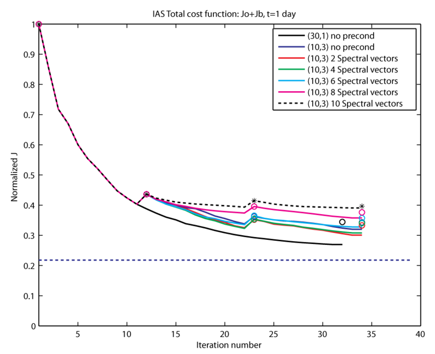
Figure 1 shows the value of $J$ computing using (1) for several different configurations of inner-loops and outer-loops for a 1 day assimilation interval. In Fig. 1, $J$ has been normalized by its initial value. For convenience, the notation $(m,n)$ is used where $n$ is the number of outer-loops employed, and $m+1$ is the number of inner-loops per outer-loop. The inner-loop count is $m+1$ rather than $m$ because the first inner-loop of each outer-loop acts as an important initialization step for the Lanczos vector sequence. The total number of iterations performed is $(m+1)n$.

The curves in Fig. 1 show the cost function computed using (1) using the increments from the inner-loops. However, a much more important practical indicator of the overall performance of the data assimilation system is the cost function, $J_{\rm {NL}}^{k}$, computed directly from the NLROMS solution during each outer-loop. Using the previous notation:

$$J_{\rm {NL}}^{k}={\frac {1}{2}}({\bf {x}}^{k}-{\bf {x}}_{b})^{T}{\bf {B}}^{-1}({\bf {x}}^{k}-{\bf {x}}_{b})+{\frac {1}{2}}({\cal {G}}({\bf {x}}^{k})-{\bf {y}})^{T}{\bf {O}}^{-1}({\cal {G}}({\bf {x}}^{k})-{\bf {y}})$$

(4)

The values of normalized $J_{\rm {NL}}^{k}$ are indicated in Fig. 1 as the color-coded symbols $\circ$ or *. The dashed horizontal line in Fig. 1 represents the theoretical minimum value of $J$ given by half the number of observations assimilated during the 1-day interval.

For reference, two unpreconditioned I4DVAR calculations are shown in Fig. 1 corresponding to (30,1) and (10,3). The remaining curves in Fig. 1 show the evolution of $J$ for (10,3) using spectral preconditioning and different numbers of the estimated eigenvectors ${\bf {u}}_{i}$ of the Hessian matrix ${\bf {A}}$. In all cases, the solution is identical for the first 10 iterations because second level preconditioning is only applied beyond that point. The estimated accuracy $\epsilon$ varies between $O(10^{-6})$ for ${\bf {u}}_{1}$ and ${\bf {u}}_{2}$ and $O(10^{-2})$ for ${\bf {u}}_{i},~~i=[2,10]$. Figure 1 reveals that as the number of eigenvectors used increases from 2 to 10, the values of $J$ and $J_{\rm {NL}}$ increase, indicating that using the less accurate vectors ${\bf {u}}_{i}$ degrades the convergence rate of the cost function. This is in agreement with Tshimanga et al. (2008). The acceptable accuracy of the eigenvectors is controlled by the ROMS input parameter HevecErr, and the experiments in Fig. 1 suggest that HevecErr should be chosen to be $<10^{-2}$. The best case shown in Fig. 1 corresponds to using 2 eigenvectors. On first inspection, Fig. 1 suggests that the unpreconditioned case (30,1) produces the best solution. This is certainly true for $J$, however for the more important measure $J_{\rm {NL}}$, the spectrally preconditioned (10,3) case using 2 eigenvectors is superior.

Figure 2: The normalized cost function $J$ computed within inner-loops (curves), and $J_{NL}$ the cost function computed relative to the nonlinear model during outer-loops (open circles). The various cases shown are for a 1-day assimilation window: (30,1) no preconditioning (solid black line, black circles); (10,3) no preconditioning (solid dark blue line, dark blue circles); (10,3) and Ritz preconditioning using 2 Ritz vectors (red curve, red circles), 4 Ritz vectors (green curve, green circles), 6 Ritz vectors (turquoise line, turquoise circles), 8 Ritz vectors (purple line, purple circles), and 10 Ritz vectors (black dashed curve, black asterisks).The horizontal dashed blue line represents the theoretical minimum value of the cost function given by half the number of assimilated observations.

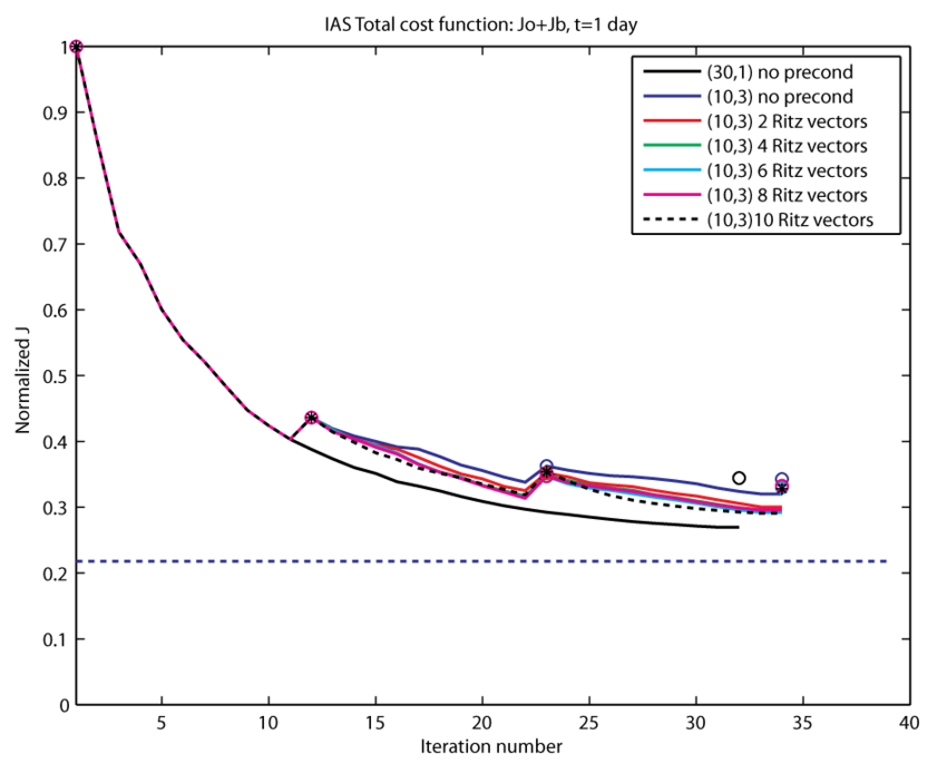
Figure 2 has the same format as Fig. 1 and shows instead the case where Ritz preconditioning is employed using different numbers of Ritz vectors. As discussed by Tshimanga et al. (2008), the Ritz preconditioner is less sensitive to the accuracy $\epsilon$ of the Ritz vectors ${\bf {z}}_{i}$ that are used. This is also the case in Fig. 2 where increasing the number of vectors ${\bf {z}}_{i}$ used leads to a continual increase in the rate of convergence of $J$ and $J_{\rm {NL}}$, despite the fact that $\epsilon$ for each ${\bf {z}}_{i}$ is quite large for $i>2$. In fact, (10,3) using all 10 available ${\bf {z}}_{i}$ is the best case in Fig. 2 both in terms of $J$ and $J_{\rm {NL}}$.

Figure 3: The normalized cost function $J$ computed within inner-loops (curves), and $J_{NL}$ the cost function computed relative to the nonlinear model during outer-loops (open circles). The various cases shown are for a 1-day assimilation window: (10,3) and Ritz preconditioning using 2 Ritz vectors (black curve, black circles), and 10 Ritz vectors (red curve, red asterisks); and (10,3) and spectral preconditioning using 2 eigenvectors (blue line, blue circles). The horizontal dashed blue line represents the theoretical minimum value of the cost function given by half the number of assimilated observations.

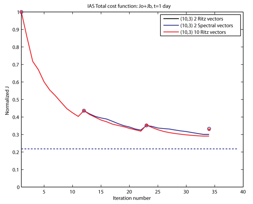
Inspection of equations (2) and (3) shows that the spectral and Ritz preconditioners are similar except that the Ritz preconditioner possesses an additional term which accounts for the formal error in the Ritz vector estimates. Therefore, if both preconditioners are restricted to using only accurate eigenvectors (i.e. small $\epsilon$), both should yield very similar results because the last term in equation (3) will be small. This is confirmed in Fig. 3 which shows $J$ and $J_{\rm {NL}}$ for (10,3) using spectral and Ritz preconditioning with 2 eigenvectors - the two cases are indistinguishable. Figure 3 also shows the (10,3) case using Ritz preconditioning and 10 Ritz vectors, and indicates that while $J$ is significantly smaller than the case using only 2 vectors, the percentage reduction in $J_{\rm {NL}}$ is not nearly as marked.

Ritz Preconditioning and Iteration Dependence

The results from the previous section indicate that Ritz preconditioning is generally superior to spectral preconditioning and more robust in the sense that it is less sensitive to the accuracy $\epsilon$ of the eigenvectors that are admitted to the preconditioners. In this section the sensitivity of the Ritz preconditioner to the combination of inner- and outer-loops is considered.

Figure 4: The normalized cost function $J$ computed within inner-loops (curves), and $J_{NL}$ the cost function computed relative to the nonlinear model during outer-loops (open circles). The various cases shown are for a 1-day assimilation window: (30,1) no preconditioning (solid black line, black circles); (10,3) no preconditioning (solid dark blue line, dark blue circles); (10,3) and Ritz preconditioning using 10 Ritz vectors (dashed black curve, black asterisks); (15,2) and Ritz preconditioning using 15 Ritz vectors (green curve, green circles); and (5,6) and Ritz preconditioning using 4 Ritz vectors (red curve, red circles).The horizontal dashed blue line represents the theoretical minimum value of the cost function given by half the number of assimilated observations.

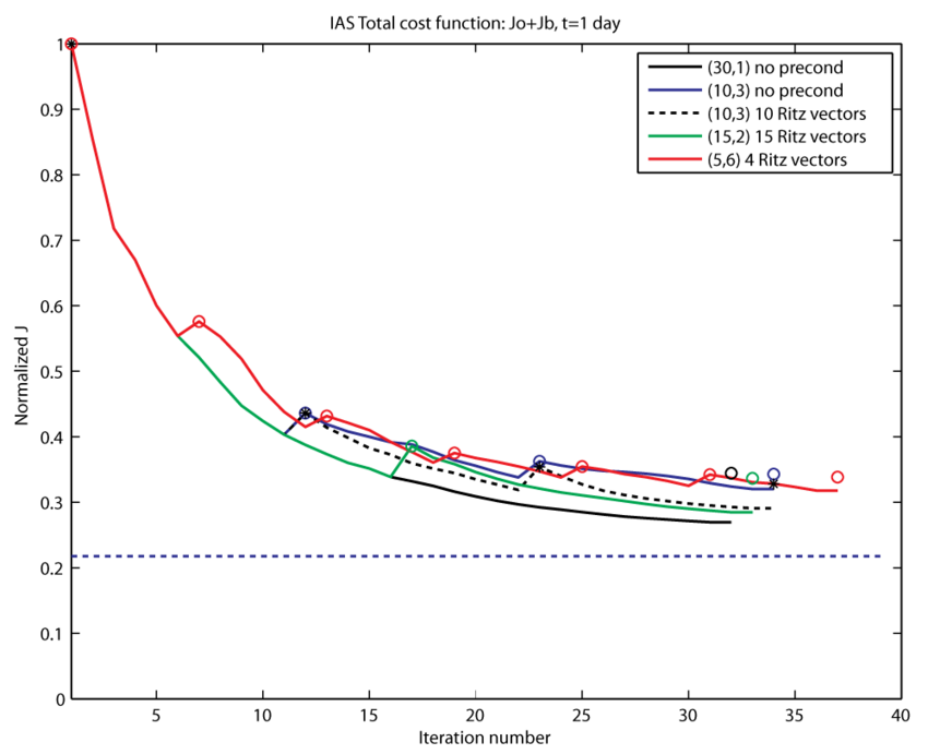
Figure 4 shows $J$ and $J_{\rm {NL}}$ for 1-day cases for which the total number of iterations is similar ($\sim 30-36$) but which employ different combinations of inner- and outer-loops. The computational effort is therefore comparable in all cases. The (30,1) and (10,3) reference cases that use no preconditioning are included in Fig. 4. The best case identified in section 3.1 was (10,3) with Ritz preconditioning using all 10 Ritz vectors from outer-loops $k=2$ and $k=3$. This case is reproduced in Fig. 3, along with a (15,2) case and a (5,6) case. In the (15,2) case there are 15 Ritz vectors available for preconditioning during the 2nd outer-loop, and Fig. 4 shows that while $J$ is lower than the (10,3) case at the end of the experiment, the (10,3) case is still superior based on $J_{\rm {NL}}$. During the (5,6) case there are potentially 6 Ritz vectors available, during outer-loops $k=[2,5]$, but in general only 4 of them have sufficiently small $\epsilon$ to be useful. Each iteration of the Lanczos algorithm yields not only an additional Ritz vector, but also refines the estimates of those Ritz vectors identified during previous inner-loops. Therefore, $\epsilon$ decreases for all of the Ritz vectors as the number of inner-loops increases. Attempts to use all 6 Ritz vectors lead to significant degradation of $J$ and $J_{\rm {NL}}$ (not shown). Figure 4 shows the (5,6) case using 4 Ritz vectors which does not perform as well as (10,3) or (15,2) and is similar to the case with no preconditioning.

Figure 4 suggests that for a given computational effort (as dictated by the combined number of innner- and outer-loops), Ritz preconditioning is most effective with $k>2$ and $m\sim 10$. This reflects the trade-off between the increased accuracy of the available Ritz vectors with increasing number of inner-loops, and the benefits of updating the non-linear ROMS solution about which the inner-loop minimizations are performed.

Dependence on Assimilation Time Window

Figure 5: The normalized cost function $J$ computed within inner-loops (curves), and $J_{NL}$ the cost function computed relative to the nonlinear model during outer-loops (open circles). The various cases shown are for a 3-day assimilation window: (30,1) no preconditioning (solid black curve, black circles); (10,3) no preconditioning (solid dark blue line, dark blue circles); (10,3) and spectral preconditioning using 2 eigenvectors (red curve, red circles), and 10 eigenvectors (green curve, green circles); (10,3) and Ritz preconditioning using 5 Ritz vectors (turquoise line, turquoise circles), and 10 Ritz vectors (black dashed curve, black asterisks). The horizontal dashed blue line represents the theoretical minimum value of the cost function given by half the number of assimilated observations.

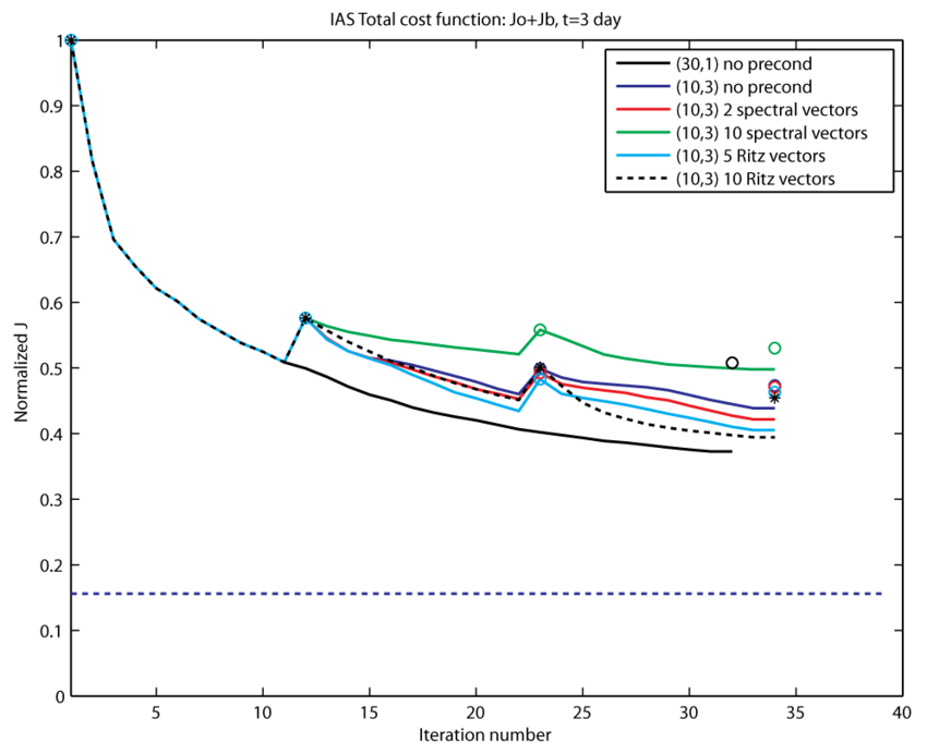
A subset of the experiments presented in the previous 2 sections were repeated using 3-day and 7-day assimilation windows. The results for the 3-day case are shown in Fig. 5. Figure 5 shows results from two spectrally preconditioned (10,3) cases, one employing 2 eigenvectors and the other 10 eigenvectors. As in the 1-day case, the performance of spectral preconditioning is degraded by using inaccurate estimates of the Hessian eigenvectors. The 2 eigenvector case, however, is superior to the (30,1) case with no preconditioning, but only marginally better than (10,3) case with no preconditioning. Two (10,3) cases using Ritz preconditioning and 5 and 10 Ritz vectors respectively are also shown in Fig. 5. The latter is the best case of all for $J_{\rm {NL}}$.

Figure 6: The normalized cost function $J$ computed within inner-loops (curves), and $J_{NL}$ the cost function computed relative to the nonlinear model during outer-loops (open circles). The various cases shown are for a 7-day assimilation window: (30,1) no preconditioning (solid black curve, black circles); (10,3) no preconditioning (solid dark blue line, dark blue circles); (10,3) and spectral preconditioning using 2 eigenvectors (red curve, red circles), (10,3) and Ritz preconditioning using 5 Ritz vectors (green curve, green circles); and 10 Ritz vectors (black dashed curve, black asterisks). The horizontal dashed blue line represents the theoretical minimum value of the cost function given by half the number of assimilated observations.

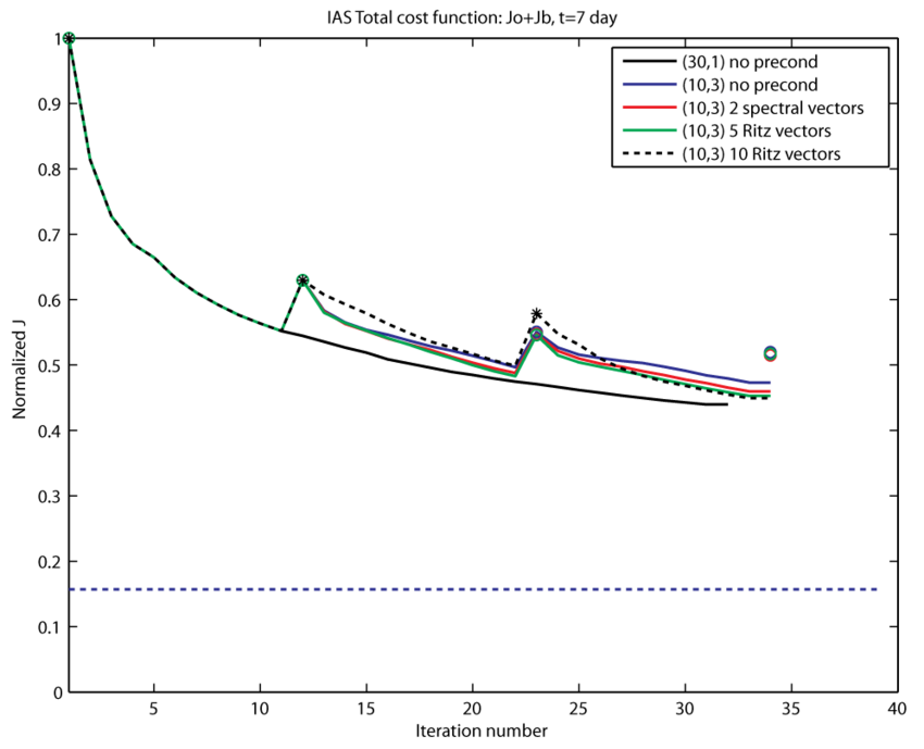
The results from the same combinations of inner- and outer-loops and preconditioners using a 7-day assimilation window are shown in Fig. 6. In this case, some of the $J_{\rm {NL}}$ values are missing at the end of the final outer-loop for some of the calculations because the initial condition generated by I4DVAR caused the model to blow-up. This is indicative that a 7-day assimilation combined with a large combined number of inner- and outer-loops may be pushing the tangent linear assumption beyond what is a reasonable limit. Figure 6 suggests that while $J$ sometimes shows a significant improvement with preconditioning, the assimilation scheme is struggling to converge. The values of $\epsilon$ for the eigenvectors and Ritz vectors in this case are consistently higher than for the 1-day and 3-day cases, so the uninspiring performance of the preconditioners in the 7-day case may be due partly to the lower accuracy of the available vectors and partly to violation of the tangent linear assumption.

Summary and Recommendations

The preconditioned Lanczos-method based I4DVAR scheme has been successfully implemented in the ROMS code. The experiments described above indicate that the algorithm is working correctly. Two types of second level preconditioning are available: so-called spectral preconditioning in which estimates of the Hessian eigenvectors are used; and Ritz preconditioning in which the Ritz vectors of the Hessian are used. Although not explicitly stated or obvious from the above discussion, the Hessian eigenvectors estimates and Ritz vectors are identical, so the only difference between the two approaches to preconditioning is the way in which the eigenvector information is used. As discussed in the Spectral vs Ritz preconditioning section, the accuracy of the Hessian eigenvectors ${\bf {u}}_{i}$ that are employed in the spectral preconditioner is a critical factor: using eigenvectors for which $\epsilon$ is too large degrades the performance of I4DVAR. The Ritz preconditioner of Tshimanga et al. (2008), however, cleverly circumvents this problem by accounting for the formal error in the eigenvectors (now referred to as the Ritz vectors).

While the above experiments are far from exhaustive, they do give some sense of the performance that can be expected from preconditioned I4DVAR system. Based on these experiments, the following recommendations can be considered as providing useful guidance for configuring the ROMS I4DVAR system and choosing the preconditioner parameters:

1. For spectral preconditioning, it is recommended that the threshhold for acceptable accuracy of the Hessian eigenvectors estimates, HevecErr be chosen to be $\leq 10^{-3}-10^{-4}$.
2. For Ritz preconditioning, Ritz vectors of relatively low accuracy can be tolerated, so HevecErr $\leq 10^{-1}-10^{-2}$ is recommended.
3. For any problem there will be a maximum acceptable computational cost which will dictate the total number of inner-loops and outer-loops that can be used. There is a trade-off between the number of inner-loops and outer-loops in that increasing the number of inner-loops yields more eigenvectors or Ritz vectors of acceptable accuracy for the preconditioner, while increasing the number of outer-loops allows more frequent updating of the NLROMS solutions which helps to drive down $J_{\rm {NL}}$. The recommendation here is that the number of inner-loops be at least 10, and that the number of outer-loops be at least 3.
4. The experience here is that a long assimilation window can degrade the performance of the preconditioner. This needs to be more fully explored, but is probably associated with violation of the tangent linear assumption when the assimilation window is excessively long.