 652) and recompute the input nesting grid connectivity (NGC) NetCDF file generated by contact.m.
 Nesting Algorithm Update for Refinement Grids Super-Class
The nesting algorithms were improved to include various types of refinement configurations (svn trunk revision 747) as shown in
Definitions:
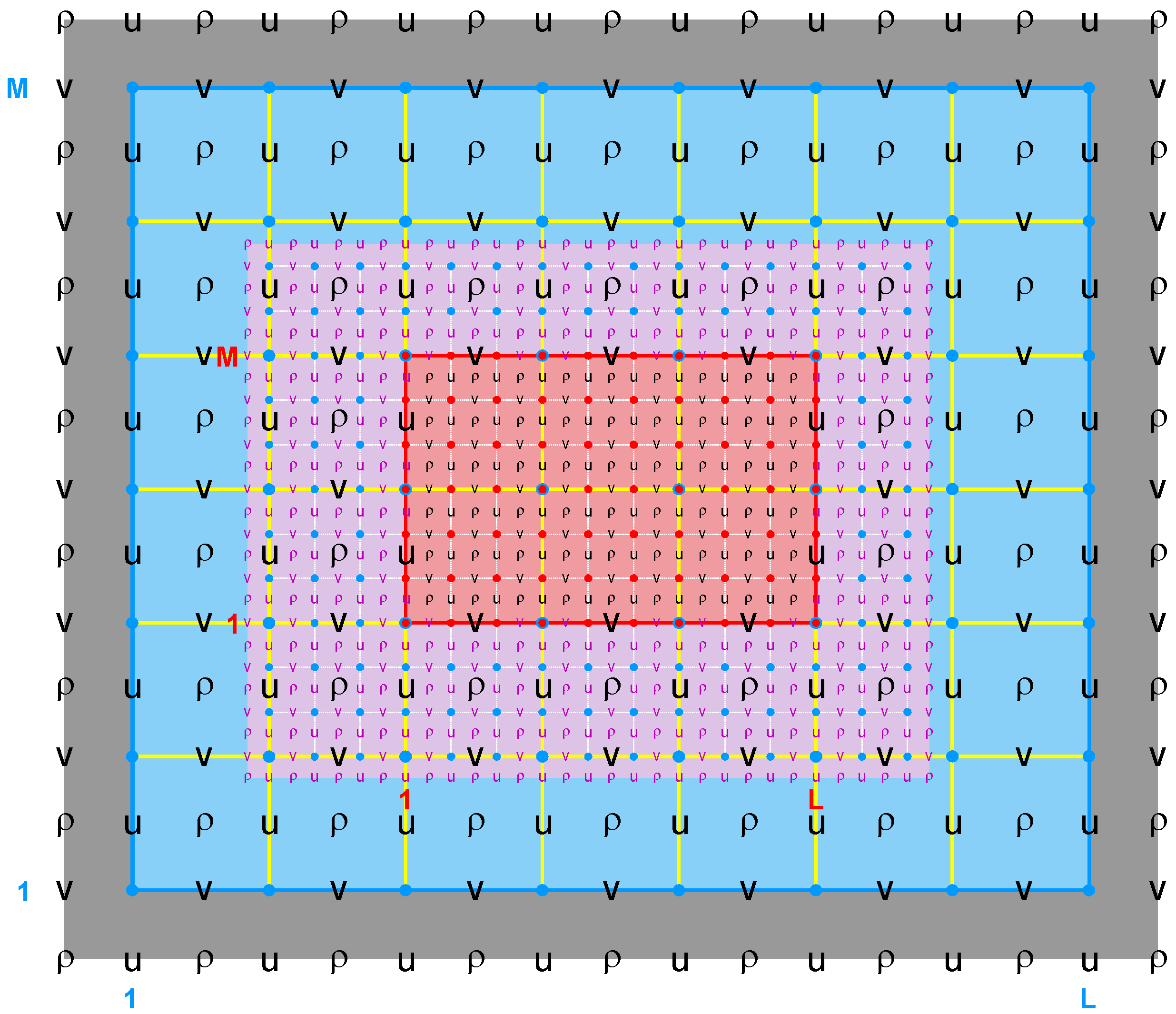
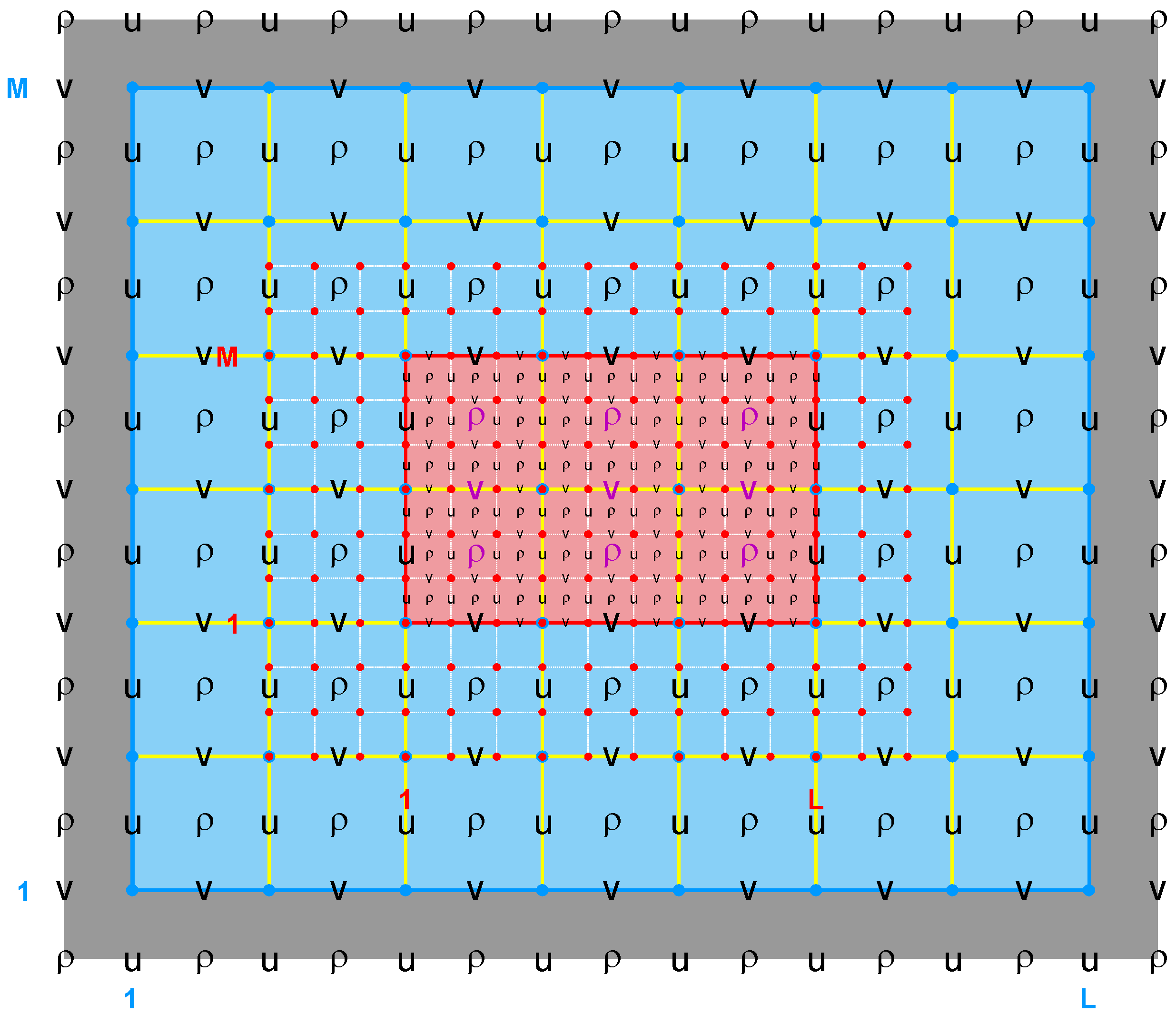
- Contact Region (cr): Extended section of the nested grid that overlays an adjacent nested grid. It is the region where the exchange of data between nested grids takes place. Since ROMS nesting is two-way by default, there are Ncontact=(Ngrids-1)*2 contact regions, where Ngrids is the number of nested grids and Ncontact is the number of contact regions in a nested application. The above diagram shows a contact region (left panel; purple) where the coarser donor grid (blue) is used to interpolate the contact points data for the finer receiver grid (red). The right panel shows its associated conjugate contact region used in two-way nesting to feedback (spatial averaging) data from fine to coarse grids. Notice the duality of a ROMS nested grid: data donor in one contact region and data receiver in its conjugate contact region. This explains why we prefer to use the donor and receiver categories instead of the usual parent and child descriptions found in the literature. Each contact region has a donor and a receiver grid.
- Contact Points: Grid cells inside a contact region. Since ROMS governing equations are solved in an Arakawa C-grid, there are contact points at ρ-, Ψ-, u-, and v-points. However, the Ψ-points are only used to define the physical grid perimeters within a contact region. ROMS nesting is unique in the sense that the full horizontal operators are evaluated at the contact points between nested grids instead of specifying a value and flux at the nested grid physical boundary edge. This is similar to what is done in periodic boundary conditions and distributed-memory parallel tile exchanges. Notice that since the C-grid stencil indices in ROMS are left-bottom ordered (that is, the u to the left of ρ and the v to the bottom of ρ have the same (i,j) indices), there are always 4 ρ contact points at the left and bottom side of the contact region. On the other hand, there a 3 ρ contact points on the right and top side of the contact region.
- Donor Grid (dg): Data source grid in a nesting contact region. In refinement, the donor grid is used either to interpolate data from coarse to fine grid or to average data from fine to coarse grid (two-way feedback).
- Receiver Grid (rg): Data recipient grid in a nesting contact region. In refinement, the contact points of the finer receiver grid are interpolated using the coarser donor data from the grid cell containing the contact point. The interpolation can be linear or quadratic. The quadratic conservative interpolation is not fully implemented and will be available in the future. In two-way nesting, when the coarse grid is the receiver grid the finer grid solution is averaged within the coarse cell. The coarse grid cell value is replaced with the finer grid averaged solution. This takes place in routine fine2coarse.
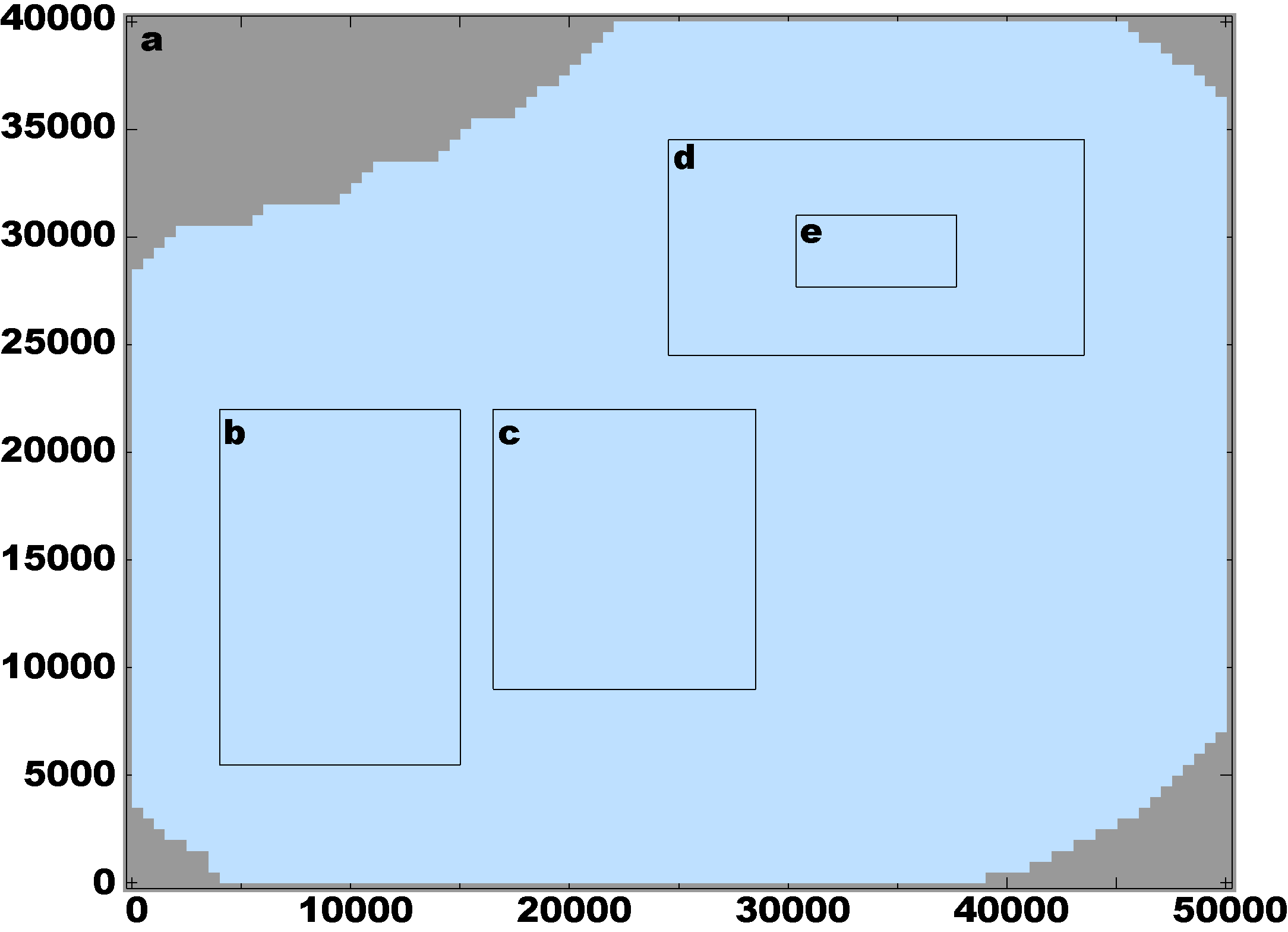
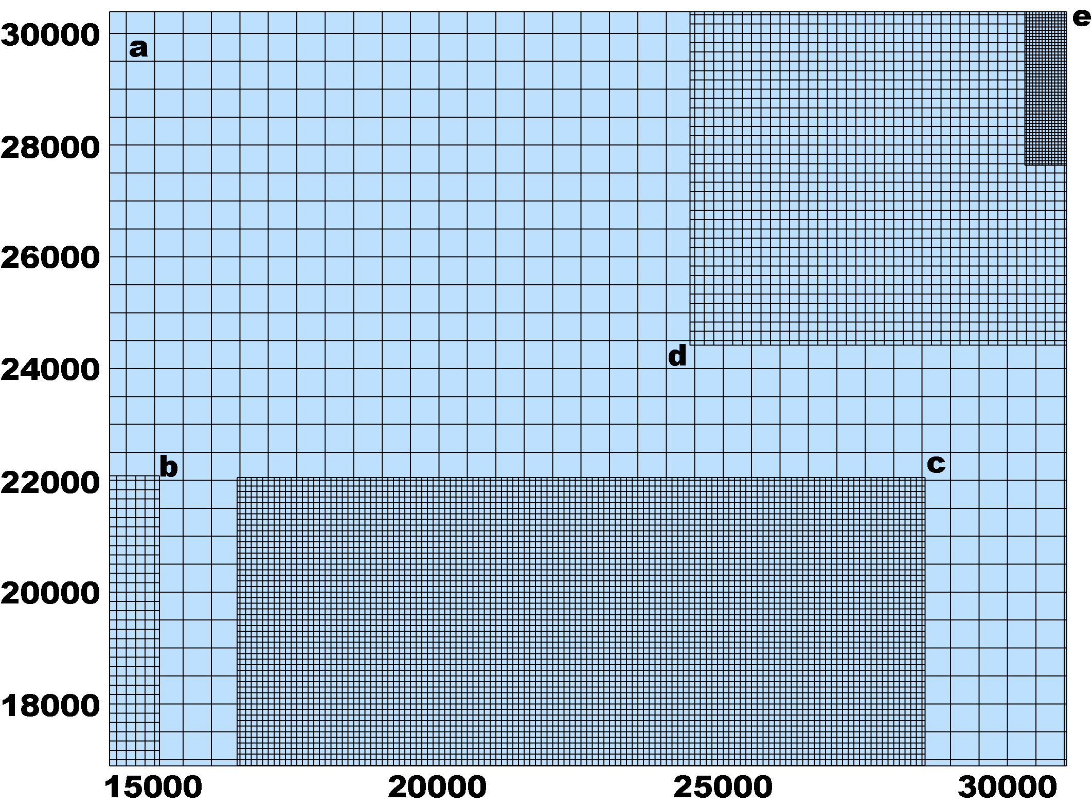
- Telescoping Grid: Technically, inside ROMS a telescoping grid is a refined grid, with RefineScale > 0, including another finer refined grid inside. In the diagram below for LAKE_JERSEY, grid d is the telescoping grid. Outside ROMS is clear that a, d, and e have a telescoping arrangement.
- Nesting Layer: Nested grids time-step arrangement and order for the ROMS numerical kernel. It is directly related to the time-step size (dt) for each nested grid. The number of nested layers, NestLayers, is specified in standard input script (ocean.in) and should be equal to the different number of time-step size (dt). For example, the
 Lake Jersey Examples include various Nesting Layer arrangements:
Code: Select all
      Grids Considered       NestLayers       GridsInLayer        WikiROMS Example

          a, b                   2               1, 1              Lake Jersey AB
          a, c                   2               1, 1              Lake Jersey AC
          a, d                   2               1, 1              Lake Jersey AD
          a, b, d                2               1, 2              Lake Jersey ABD
          a, d, e                3               1, 1, 1           Lake Jersey ADE
          a, b, d, c             3               1, 2, 1           Lake Jersey ABDC
          a, c, d, e             4               1, 1, 1, 1        Lake Jersey ACDE
What Is New:
- Fixed the mass flux in put_refine2d by providing the appropriate donor coarser grid values of DU_avg2 and DV_avg2 at the correct finer grid contact points. The latest values of these coarser grid transports are imposed at the physical boundary of the refined grid. A new routine, get_persisted2d, is used to fill the transport values REFINED(cr)%DU_avg(1,:,tnew) and REFINED(cr)%DV_avg(1,:,tnew). The sum of the refined grid fluxes is equal to the value of the coarse grid cell containing them.
- Similar mass flux is imposed a every predictor and corrector barotropic time-step in u2dbc_im.F and v2dbc_im.F but the transport is adjusted with the latest value of zeta(:,:,kout) to conserve mass and volume. Many thanks to John Warner for bringing this to my attention.
- A new diagnostic routine check_massflux was coded to check the mass fluxes between coarse and fine grids for mass and volume conservation. The transport values for both coarse and fine grids are stored in BOUNDARY_CONTACT(:,cr)%mflux(:) in their respective contact regions. If the C-preprocessing option NESTING_DEBUG is activated, it will write very verbose ASCII data into Fortran unit 300 (usually file fort.300). You will get something like:
Code: Select all
Western Boundary Mass Fluxes: cr = 01 dg = 01 rg = 02 iif(rg) = 001 iic(rg) = 0000001 time(rg) = 0000000 Coarse Coarse Grid Fine Grid Ratio Jb DU_avg2 SUM(DU_avg2) 0050 2.30201792E+00 2.30201792E+00 1.00000000E+00 0051 2.30201792E+00 2.30201792E+00 1.00000000E+00 0052 2.30201792E+00 2.30201792E+00 1.00000000E+00 0053 2.30201792E+00 2.30201792E+00 1.00000000E+00 0054 2.30201792E+00 2.30201792E+00 1.00000000E+00 0055 2.30201792E+00 2.30201792E+00 1.00000000E+00 0056 2.30201792E+00 2.30201792E+00 1.00000000E+00 0057 2.30201792E+00 2.30201792E+00 1.00000000E+00 0058 2.30201792E+00 2.30201792E+00 1.00000000E+00 0059 2.30201792E+00 2.30201792E+00 1.00000000E+00 0060 2.30201792E+00 2.30201792E+00 1.00000000E+00 0061 2.30201792E+00 2.30201792E+00 1.00000000E+00 0062 2.30201792E+00 2.30201792E+00 1.00000000E+00 0063 2.30201792E+00 2.30201792E+00 1.00000000E+00 0064 2.30201792E+00 2.30201792E+00 1.00000000E+00 0065 2.30201792E+00 2.30201792E+00 1.00000000E+00 0066 2.30201792E+00 2.30201792E+00 1.00000000E+00 0067 2.30201792E+00 2.30201792E+00 1.00000000E+00 0068 2.30201792E+00 2.30201792E+00 1.00000000E+00 0069 2.30201792E+00 2.30201792E+00 1.00000000E+00 ... and so on - Usually, the time-step size of the receiver refined grid , dt(rg), needs to be a RefineScale factor smaller than the coarser donor grid time-step, dt(dg). This restriction is now relaxed to be an exact multiple of the coarser grid value. We just need to satisfy: MOD[dt(dg), dt(rg)] = 0. That is, you can take a smaller or larger dt(rg) than the one dictated by the global grid stability, dt(rg) = dt(dg) / RefineScale.
- Changed how the contact points interpolation weights (Lweight and Qweight) are computed in the Matlab script contact.m. No longer they are adjusted to take into account the land/sea mask at contact points. This is now done in ROMS new routine mask_hweights to facilitate computations when wetting and drying (WET_DRY) is activated. In wetting and drying, the land/sea mask evolves at every time step and these masks are not available to be used in contact.m and the time dependency is a problem. Only the permanent land/sea masking arrays are available for this script.
- The NESTING_DEBUG C-preprocessing option is for developers and very curious users.
 The model should be run for only couple of time-steps of Grid ng=1 (coarser grid in your application). I usually run this in serial or on a couple of parallel processors. Please do not run this in more than four parallel processors. Additional information is also written to Fortran units 100 (fort.100) and 200 (fort.200). In unit 100, there is information about the indices used to extract coarse grid data in routine get_refine and stored in structure REFINED(cr):
In unit 200, there is information about the time interpolation weights used in put_refine:
The model should be run for only couple of time-steps of Grid ng=1 (coarser grid in your application). I usually run this in serial or on a couple of parallel processors. Please do not run this in more than four parallel processors. Additional information is also written to Fortran units 100 (fort.100) and 200 (fort.200). In unit 100, there is information about the indices used to extract coarse grid data in routine get_refine and stored in structure REFINED(cr):
In unit 200, there is information about the time interpolation weights used in put_refine:Code: Select all
ng cr dg rg iic iic told tnew Tindex Tindex time time time (dg) (rg) 2D 3D told tnew (ng) 1 1 1 2 1 0 2 1 1 2 0 0 0 1 2 1 3 1 0 2 1 1 2 0 0 0 1 1 1 2 1 0 1 2 2 2 0 90 0 1 2 1 3 1 0 1 2 2 2 0 90 0 3 5 3 4 1 0 2 1 1 2 0 0 0 3 5 3 4 1 0 1 2 2 2 0 30 0 3 5 3 4 2 3 2 1 2 1 30 60 30 3 5 3 4 3 6 1 2 2 2 60 90 60 1 1 1 2 2 5 2 1 2 1 90 180 90 1 2 1 3 2 3 2 1 2 1 90 180 90Again, this information is very verbose and you have been warnedCode: Select all
cr dg ng iic iic told tnew time time time Wold Wnew (dg) (ng) (ng) told tnew 1 1 2 1 1 1 2 0 0 90 1.0000 0.0000 1 1 2 1 2 1 2 18 0 90 0.8000 0.2000 1 1 2 1 3 1 2 36 0 90 0.6000 0.4000 1 1 2 1 4 1 2 54 0 90 0.4000 0.6000 1 1 2 1 5 1 2 72 0 90 0.2000 0.8000 2 1 3 1 1 1 2 0 0 90 1.0000 0.0000 5 3 4 1 1 1 2 0 0 30 1.0000 0.0000 5 3 4 1 2 1 2 10 0 30 0.6667 0.3333 5 3 4 1 3 1 2 20 0 30 0.3333 0.6667 2 1 3 1 2 1 2 30 0 90 0.6667 0.3333 5 3 4 2 4 2 1 30 30 60 1.0000 0.0000 5 3 4 2 5 2 1 40 30 60 0.6667 0.3333 5 3 4 2 6 2 1 50 30 60 0.3333 0.6667 2 1 3 1 3 1 2 60 0 90 0.3333 0.6667 5 3 4 3 7 1 2 60 60 90 1.0000 0.0000 5 3 4 3 8 1 2 70 60 90 0.6667 0.3333 5 3 4 3 9 1 2 80 60 90 0.3333 0.6667 Otherwise, you will fill the computer with very large files
- A new logical function do_twoway is added to facilitate the two-way exchange between nested grids. In main3d, we have:
In Telescoping grids, this logic is not trivial since the feedback between finer and coarse grids needs to be done at the correct time-step and correct grid sequence. For example, in the Lake Jersey case shown below we need to have:
Code: Select all
# ifndef ONE_WAY ! !----------------------------------------------------------------------- ! If refinement grids, perform two-way coupling between fine and ! coarse grids. Correct coarse grid tracers values at the refinement ! grid with refined accumulated fluxes. Then, replace coarse grid ! state variable with averaged refined grid values (two-way nesting). ! Update coarse grid depth variables. ! ! The two-way exchange of infomation between nested grids needs to be ! done at the correct time-step and in the right sequence. !----------------------------------------------------------------------- ! DO il=NestLayers,1,-1 IF (do_twoway(nl,il,istep,ng)) THEN CALL nesting (ng, iNLM, n2way) END IF END DO # endifThis is color coded inCode: Select all
STEP Day HH:MM:SS KINETIC_ENRG POTEN_ENRG TOTAL_ENRG NET_VOLUME Grid C => (i,j,k) Cu Cv Cw Max Speed 0 0 00:00:00 0.000000E+00 8.810744E+01 8.810744E+01 3.600000E+10 01 (000,00,0) 0.000000E+00 0.000000E+00 0.000000E+00 0.000000E+00 DEF_HIS - creating history file, Grid 01: lake_jersey_his_a.nc WRT_HIS - wrote history fields (Index=1,1) into time record = 0000001 01 DEF_AVG - creating average file, Grid 01: lake_jersey_avg_a.nc 0 0 00:00:00 0.000000E+00 8.832187E+01 8.832187E+01 2.808000E+09 02 (000,000,0) 0.000000E+00 0.000000E+00 0.000000E+00 0.000000E+00 DEF_HIS - creating history file, Grid 02: lake_jersey_his_c.nc WRT_HIS - wrote history fields (Index=1,1) into time record = 0000001 02 DEF_AVG - creating average file, Grid 02: lake_jersey_avg_c.nc 1 0 00:00:18 2.305157E-08 8.832187E+01 8.832187E+01 2.808000E+09 02 (119,130,8) 1.337117E-04 1.265846E-07 0.000000E+00 7.433504E-04 2 0 00:00:36 9.146359E-08 8.832187E+01 8.832187E+01 2.808000E+09 02 (118,003,8) 2.449648E-04 4.541085E-07 1.022608E-04 1.361476E-03 3 0 00:00:54 2.054711E-07 8.832187E+01 8.832187E+01 2.808000E+09 02 (116,005,8) 3.545964E-04 9.588826E-07 8.745096E-05 1.979927E-03 4 0 00:01:12 3.652887E-07 8.832187E+01 8.832187E+01 2.808000E+09 02 (114,007,8) 4.645087E-04 1.661081E-06 7.173268E-05 2.598741E-03 FINE2COARSE - exchanging data between grids: dg = 02 and rg = 01 at cr = 03 0 0 00:00:00 0.000000E+00 8.832187E+01 8.832187E+01 3.420000E+09 03 (000,00,0) 0.000000E+00 0.000000E+00 0.000000E+00 0.000000E+00 DEF_HIS - creating history file, Grid 03: lake_jersey_his_d.nc WRT_HIS - wrote history fields (Index=1,1) into time record = 0000001 03 DEF_AVG - creating average file, Grid 03: lake_jersey_avg_d.nc 0 0 00:00:00 0.000000E+00 8.832187E+01 8.832187E+01 4.400000E+08 04 (000,00,0) 0.000000E+00 0.000000E+00 0.000000E+00 0.000000E+00 DEF_HIS - creating history file, Grid 04: lake_jersey_his_e.nc WRT_HIS - wrote history fields (Index=1,1) into time record = 0000001 04 DEF_AVG - creating average file, Grid 04: lake_jersey_avg_e.nc 1 0 00:00:10 6.959677E-09 8.832187E+01 8.832187E+01 4.400000E+08 04 (131,02,8) 6.798364E-05 1.615316E-08 0.000000E+00 3.777368E-04 2 0 00:00:20 2.777576E-08 8.832187E+01 8.832187E+01 4.400000E+08 04 (130,03,8) 1.279516E-04 1.109439E-07 3.042578E-05 7.177313E-04 FINE2COARSE - exchanging data between grids: dg = 04 and rg = 03 at cr = 06 1 0 00:00:30 6.273202E-08 8.832187E+01 8.832187E+01 3.420000E+09 03 (113,02,8) 2.039125E-04 1.453791E-07 0.000000E+00 1.132997E-03 3 0 00:00:30 6.246794E-08 8.832187E+01 8.832187E+01 4.400000E+08 04 (128,05,8) 1.885273E-04 2.644876E-07 2.399886E-05 1.057567E-03 4 0 00:00:40 1.116552E-07 8.832187E+01 8.832187E+01 4.400000E+08 04 (131,02,8) 2.514380E-04 1.283163E-06 2.472931E-05 1.400478E-03 5 0 00:00:50 1.749418E-07 8.832187E+01 8.832187E+01 4.400000E+08 04 (130,03,8) 3.147309E-04 1.620478E-06 5.724897E-05 1.749841E-03 FINE2COARSE - exchanging data between grids: dg = 04 and rg = 03 at cr = 06 2 0 00:01:00 2.514723E-07 8.832187E+01 8.832187E+01 3.420000E+09 03 (112,03,8) 3.847356E-04 9.983178E-07 9.152179E-05 2.158263E-03 6 0 00:01:00 2.522627E-07 8.832187E+01 8.832187E+01 4.400000E+08 04 (128,01,8) 3.772862E-04 1.692145E-06 4.848581E-05 2.102508E-03 7 0 00:01:10 3.447488E-07 8.832187E+01 8.832187E+01 4.400000E+08 04 (126,60,8) 4.403682E-04 3.378879E-06 4.192504E-05 2.446613E-03 8 0 00:01:20 4.514873E-07 8.832187E+01 8.832187E+01 4.400000E+08 04 (130,02,8) 5.016708E-04 3.203450E-06 5.328500E-05 2.788662E-03 FINE2COARSE - exchanging data between grids: dg = 04 and rg = 03 at cr = 06 FINE2COARSE - exchanging data between grids: dg = 03 and rg = 01 at cr = 04 1 0 00:01:30 4.998866E-07 8.810744E+01 8.810744E+01 3.600000E+10 01 (020,63,8) 5.528460E-04 1.941304E-05 0.000000E+00 3.148106E-03 WikiROMS to facilitate reading. Notice the FINE2COARSE message from ROMS standard output. The two-way feedback needs to be done at the correct time-step and in the right sequence. Here, grid c completes 5 time-steps and then feeds back to grid a, grid d exchanges information with grid c every 3 time-steps after grid c performs a single time-step. This is done 3 times in a row because the refinement ratio between grids c and d is 1:3. Then, grid c exchanges information with grid a. This is the first thing that you need to check in an application with Telescoping Grids. - The one-way nesting activated with C-preprocessing option ONE_WAY is now working There is no longer a need to force mass and volume conservation in an engineering way
 which affected the forcing of tides in nested grids. Again, the one-way nesting has no effect whatsoever on the coarser donor grid because there is no feedback of information.
 - Speaking of tidal forcing, you only need to force with tides in the coarser grid (ng=1). ROMS numerical kernel and nesting design will take care of the other grids inside
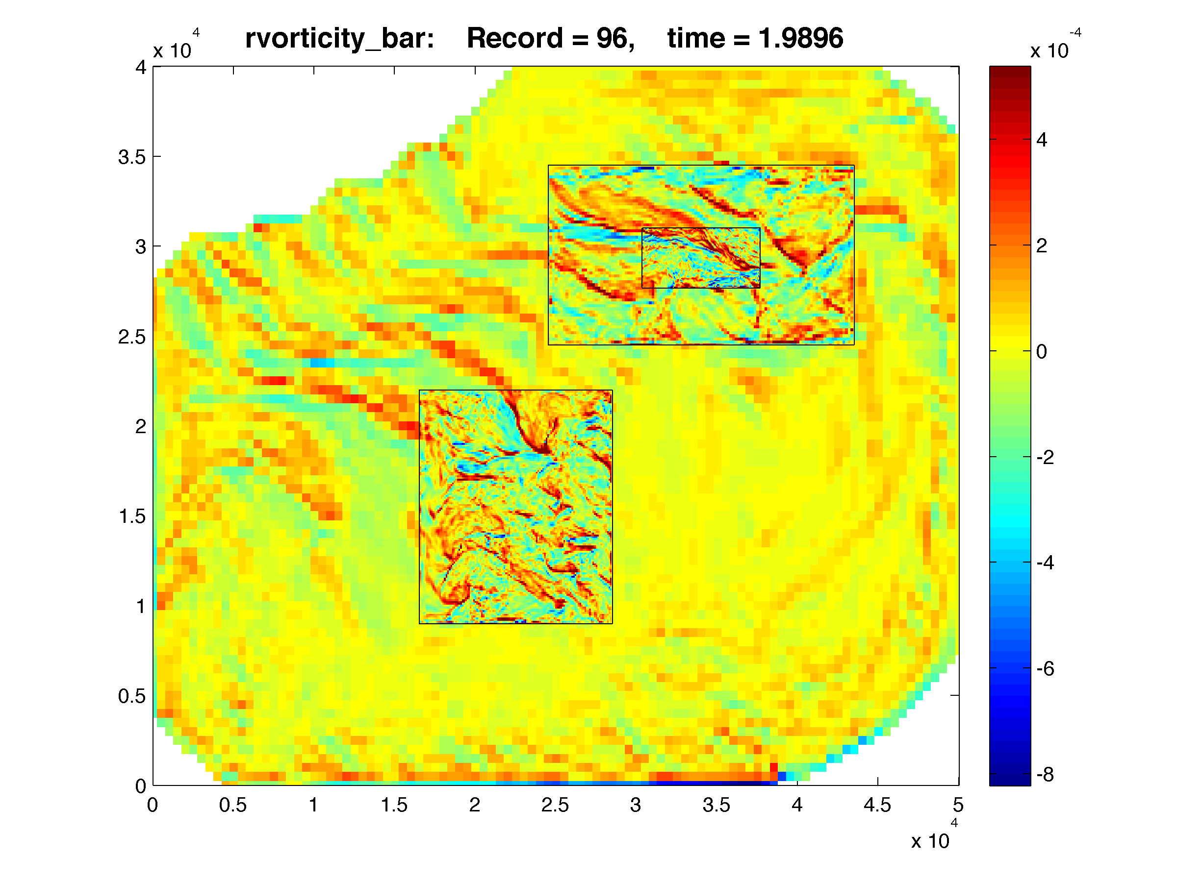
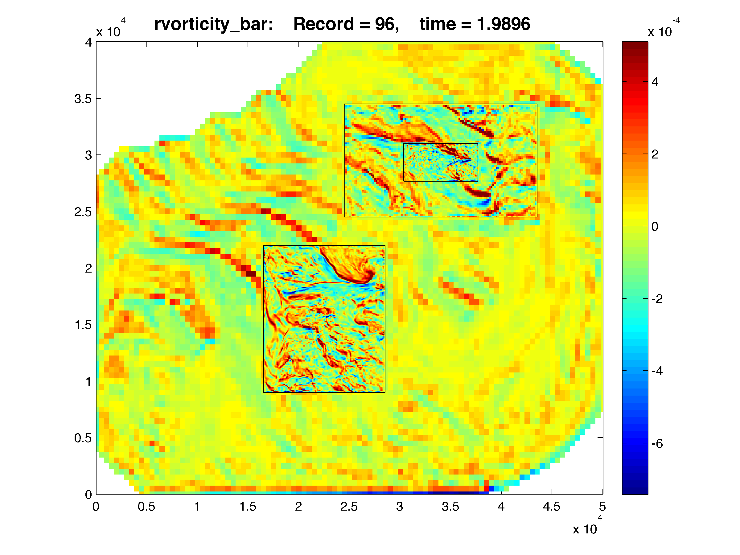
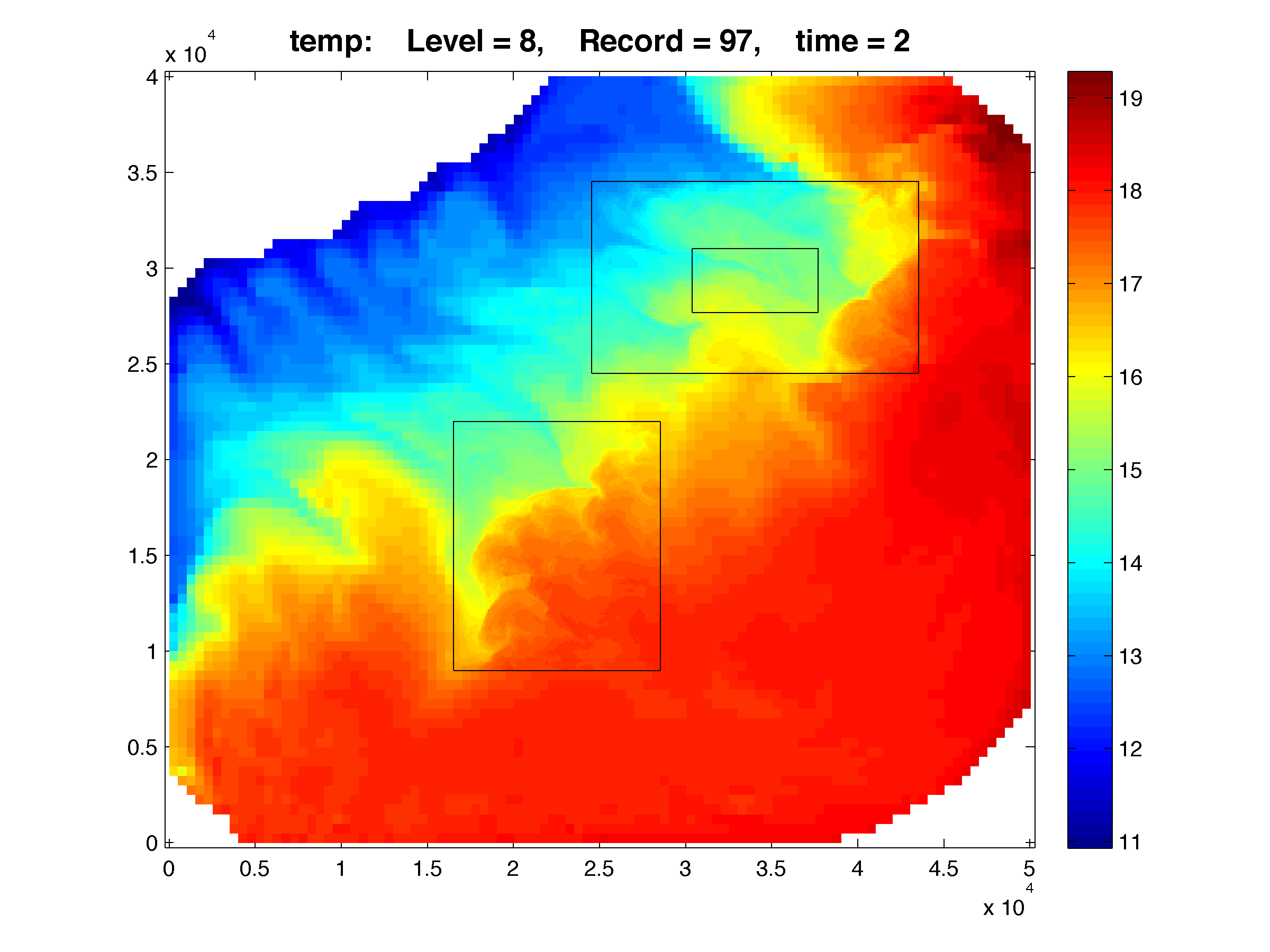
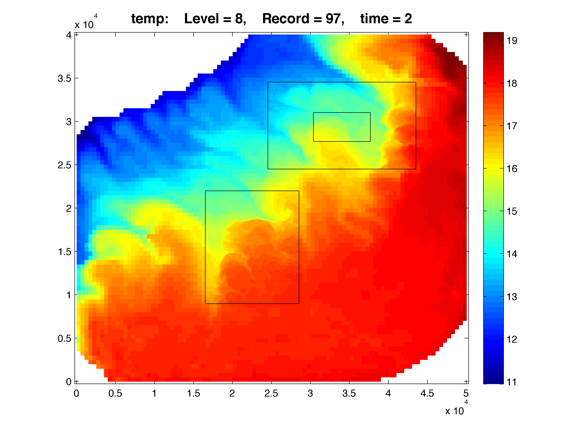
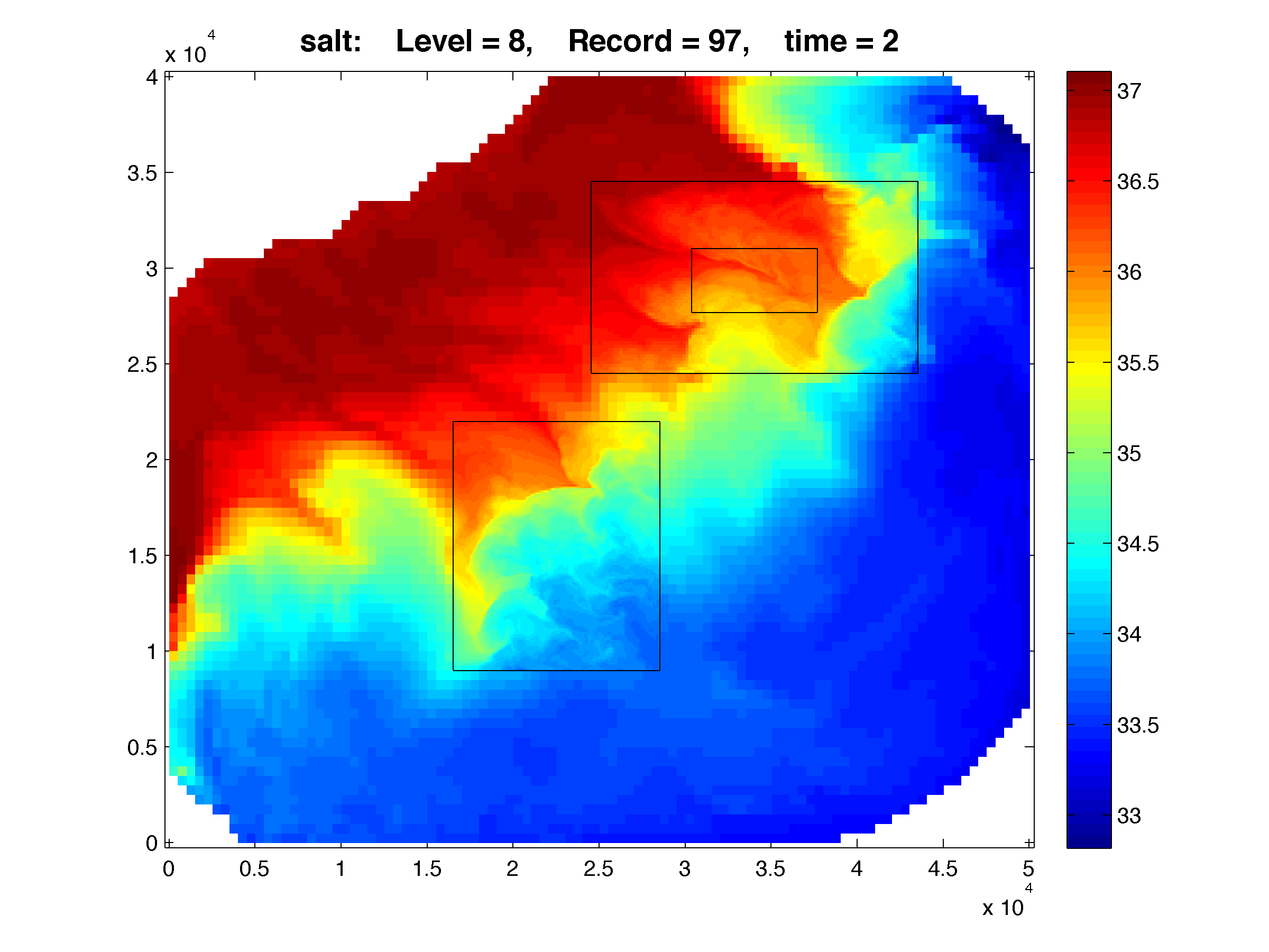
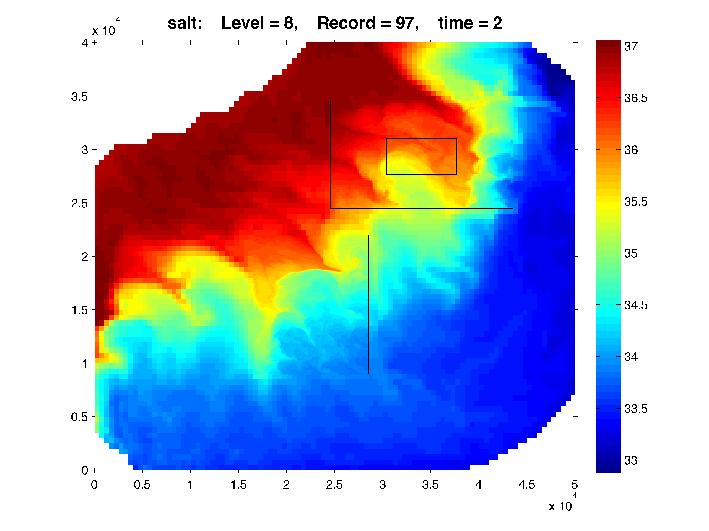
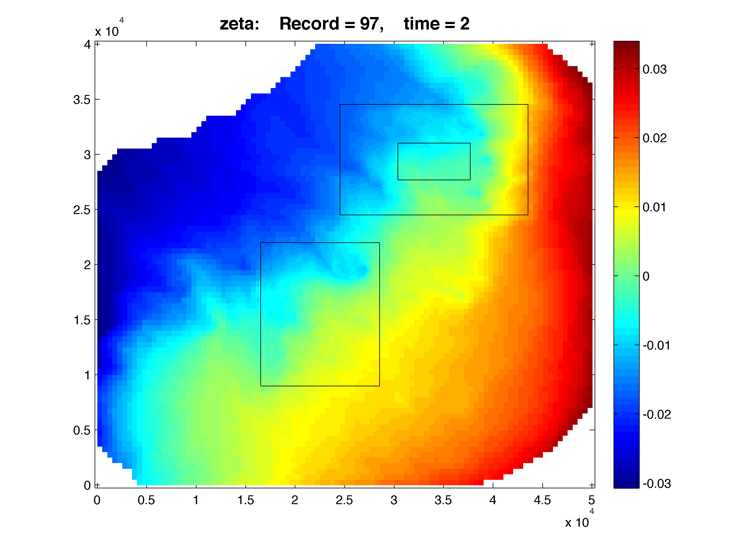
- Nesting applications with refined grids of 1:5 are working The Lake Jersey Example shown below has grid c, which is 1:5 refinement ration from grid a. The results are plotted with Matlab using the script plot_nesting.m. The refined solutions (c, and d) are overlayed on top of the coarse grid (a) and e is a overlayed on top of d. The color map is rendered using shading flat, meaning there is no interpolation between pixels in the color maps. Click the figures in WikiROMS to see a more detailed image. On the resulting page a link to the full resolution image is provided. This is ROMS version of the retina display and resolution ocean modeling
 The figures below were generated in Matlab using:
Code: Select all
 >>  Gnames = {'lake_jersey_grd_a.nc', 'lake_jersey_grd_c.nc', 'lake_jersey_grd_d.nc', 'lake_jersey_grd_e.nc'};
 >>  Anames = {'lake_jersey_avg_a.nc', 'lake_jersey_avg_c.nc', 'lake_jersey_avg_d.nc', 'lake_jersey_avg_e.nc'};
 >>  Hnames = {'lake_jersey_his_a.nc', 'lake_jersey_his_c.nc', 'lake_jersey_his_d.nc', 'lake_jersey_his_e.nc'};
 >>
 >>  G = grids_structure (Hnames, Hnames);
 >>
 >>  F = plot_nesting (G, Hnames, 'temp', 97, 8, 1, true);
 >>  F = plot_nesting (G, Hnames, 'salt', 97, 8, 1, true);
 >>  F = plot_nesting (G, Hnames, 'zeta', 97, 8, 1, true);
 >>
 >>  F = plot_nesting (G, Anames, 'rvorticity_bar', 97, 8, 1, true);
- The conservative quadratic interpolation is partially coded. The nine weights for the quadratic interpolation are now generated by the nested grid connectivity (NGC) Matlab script contact.m and stored in variable Qweights in the NGC NetCDF file. The quadratic interpolation (QUADRATIC_WEIGHTS) in ROMS will be available in the future. It cannot be activated until we recommend to do so.
- The Matlab files to generate nested grids still need some work. We need to be sure that the area between coarse and refined grids is conserved. I am planning to change the intrinsic Matlab interpolation function from TriScatteredInterp to griddedInterpolant. The function TriScatteredInterp is now obsolete. The griddedInterpolant function is available since revision R2011b.
- The nesting algorithms only work in serial and distributed-memory. In distributed-memory (MPI), we get identical solutions with 1x1, 2x2, 4x2, 3x3, and so on partitions with the C-preprocessing options tested. However in shared-memory and serial with partitions, there are parallel bugs and problems. It seems that the model is sensitive to parallel partitions in the I-direction. I will be hunting for these bugs.
- The Lagrangian drifters have not been updated to work across nested grids. It is not on the top in my priority list. Perhaps, Mark Hadfield and/or John Klinck can help us here. We need to come up with a strategy of how to do this.
- I have not tried or tested refined grids with refinement ratios of 1:7 or 1:9. I think that this is close to the limit of numerical refinement in an application.
- I have not tried or tested more than one Telescoping Grid (see definition above). I have only tested what you see below for Lake Jersey (grids a, d, and e).
- The nested algorithms are designed to work in all tracers (active and passive) since we operate on the full 5D tracer array (t). Notice that you need to have passive tracers (like biology, sediment, inert) in all the application grids since we need all the tracers data in the nesting contact points. The contact point data is computed from the donor grid, as explained above.
- If your nesting application have river runoff point sources, you may have these point sources in all the appropriate nested grids. However, you need to have a forcing river NetCDF file for each grids. Recall that the position of the point source is in (i,j) coordinates and each nested grid will have different (i,j) location values. The other river variables are the same. In principle, you can put rivers in the finer refined grid but you need two-way nesting to feedback information to the coarser grid(s).
- The more that I think about the nesting algorithms, I think that the way to build nested grids is from the fine-to-coarse grid(s) strategy. That is, we generate an intermediate grid at the finest desired resolution for the application and from it we extract the coarse grid, refined grids, and perhaps composite grids. This will give us the grid data needed for all contact points The tedious part is that we have to work the land/sea mask in a large finer-resolution intermediate grid, but it is the best representation of the coastline that we have at finest resolution. Recall that we have both coarse2fine.m and fine2coarse.m Matlab scripts for extracting nested grids. The extraction indices Imin, Imax, Jmin, and Jmax are crucial when extracting the nested grids from the intermediate fine resolution grid.
The Lake Jersey is an idealized ROMS example used primarily to test the nesting algorithms for the Refinement Grids Super-Class. It is a wind forced test with strong upwelling and upwelling plumes. The model is started from rest with uniform potential temperature and salinity. It is run for only two days for efficiency with history and time-averaged output every 30 minutes.
Various configurations of refined grids are possible including refinement ratio, telescoping grids (a, d, and e), and nesting layers. The order of the nested grids in ROMS is extremely important so several examples are shown
Code: Select all
  Grid     Mesh Size     Refinement   Donor   Donor   Donor   Donorv     Grid         Grid NetCDF File
                           Factor      Imin    Imax    Jmin    Jmax      Size

    a      100x 80x8         -           -       -       -       -      500.0 m     lake_jersey_grd_a.nc
    b       66x 99x8     1:3 from a      9      31      12      45      166.6 m     lake_jersey_grd_b.nc
    c      120x130x8     1:5 from a     34      58      19      45      100.0 m     lake_jersey_grd_c.nc
    d      114x 60x8     1:3 from a     50      88      50      70      166.6 m     lake_jersey_grd_d.nc
    e	   132x 60x8     1:3 from d     36      80      20      40       55.5 m     lake_jersey_grd_e.nc
Below is the two-day solution for example
Temperature
Salinity
Free-surface

30-minute Averaged Vertically-Integrated Relative Vorticity (1/s)