Unphysical velocities using custom salinity

Discussion of how to use ROMS on different regional and basin scale applications.

Moderators: arango, robertson

Post Reply
Message
Author
eivinds
Posts: 8
Joined: Mon Sep 28, 2009 6:08 pm
Location: Geosciences, Univ. of Oslo

Unphysical velocities using custom salinity

#1 Unread post by eivinds »

Dear ROMS community.
I am trying to simulate baroclinic wind-driven motion in a fjord in Svalbard. At the moment I try to run the model from rest with zero forcing and salinity varying in the vertical but horizontally homogenous. When i run the model there are generated unphysical currents of order 10 cm/s (!) near regions of steep topography. When I run with vertically constant salinity=32 psu, the currents are of order 2e-5 m/s which is also somewhat large...

I have tried with some different cpp-options, i.e. MIX_GEO_UV/TS, GLS_MIXING and TS_MPDATA, without significant changes. The currents are generated rather fast, after 4 hrs it is already of order 5 cm/s. Do you have any suggestions on what I am doing wrong? Must I smooth the bathymetry even more? Or is it something with my input file?

Regards,
Eivind

----------------------------
Below are some details:
The input .nc files are linked here: grid and hydrography.

My topography is manually generated and then smoothed (rfactor<0.35 everywhere). The open western boundary is closed off in the headerfile,
Image
The salinity is everywhere as the following figure (approximately, as the number of sigmalayers is finite..):
Image
After 48 hrs the u-current at sigmalayer 4 is
Image
and a vertical profile at the point of max amplitude:
Image

The .in -file is here, and below is the header file:

Code: Select all

/*
** Options for Wind-Driven internal waves in Van Mijenfjorden test
**
**
** Application flag:   VANM
** Input script:       ocean_vanm.in
*/

#define UV_ADV
#define UV_COR
#define UV_VIS2
#define UV_QDRAG
#define TS_U3HADVECTION
#define TS_C4VADVECTION
#define TS_DIF2
#define SALINITY
#define NONLIN_EOS
#define SOLVE3D
#define MASKING
#define DIAGNOSTICS_UV
#define DIAGNOSTICS_TS
#define STATIONS
#define AVERAGES
#define ANA_BSFLUX
#define ANA_BTFLUX
#define ANA_SSFLUX
#define ANA_STFLUX
#define MIX_S_UV
#define MIX_S_TS

#define MY25_MIXING
#define N2S2_HORAVG
#define KANTHA_CLAYSON

#define EASTERN_WALL
#define WESTERN_WALL
#define NORTHERN_WALL
#define SOUTHERN_WALL

#undef RST_SINGLE
#undef OUT_DOUBLE

mathieu
Posts: 74
Joined: Fri Sep 17, 2004 2:22 pm
Location: Institut Rudjer Boskovic

Re: Unphysical velocities using custom salinity

#2 Unread post by mathieu »

Dear eivinds,

yes smoothing your bathymetry is probably a good idea. But you must look at the rx1 factor, which must be around 5 or 6
at most. With the vertical stretching that impose something like rx0 around 0.18.

The key point is the error in the computation of the pressure gradient. You have an initial error, i.e. the one that you obtained but after some time the T/S distribution must stabilize to a wrong distribution but with smaller such currents and the error must then be of second type, at least according to Mellor and possibly less problematic.

The options that are relevant to the pressure gradient computation are PJ_GRAD*.

jabent
Posts: 17
Joined: Tue Jan 22, 2008 11:31 pm
Location: Australian Institute of Marine Science

Re: Unphysical velocities using custom salinity

#3 Unread post by jabent »

Hi,

Have you looked at how the density fields adjust adjacent to these regions of steep topography? The flows that you show are in the direction that one would find for a diffusively-driven flow, with an upslope Ekman transport. The strength of this flow is dependent on the slope angle and the vertical diffusivity, u ~ Kv/(delta*theta), where delta is the Ekman layer thickness. You can check if the magnitude of the flow from the model output is consistent with this scaling.

eivinds
Posts: 8
Joined: Mon Sep 28, 2009 6:08 pm
Location: Geosciences, Univ. of Oslo

Re: Unphysical velocities using custom salinity

#4 Unread post by eivinds »

Dear Community,
Thank you for your kind input.

I have worked more on my bathymetry, as I realize my rx1 number was way too high. Using GRID_SmoothPositive_ROMS_rx1.m from the LP-bathymetry package with rx1max=5 i obtained a rx0-value of 0.078 which is way lower than I need. In addition I have simplified the sigmalayer distribution to Vstretch=1, Vtrans=2, thetab=thetas=1.
The max currents are now smaller but still several cm/s. When i run without salinity differences the currents are <1e.5 cm/s everywhere so it is definetely something with how the stratification is handled.

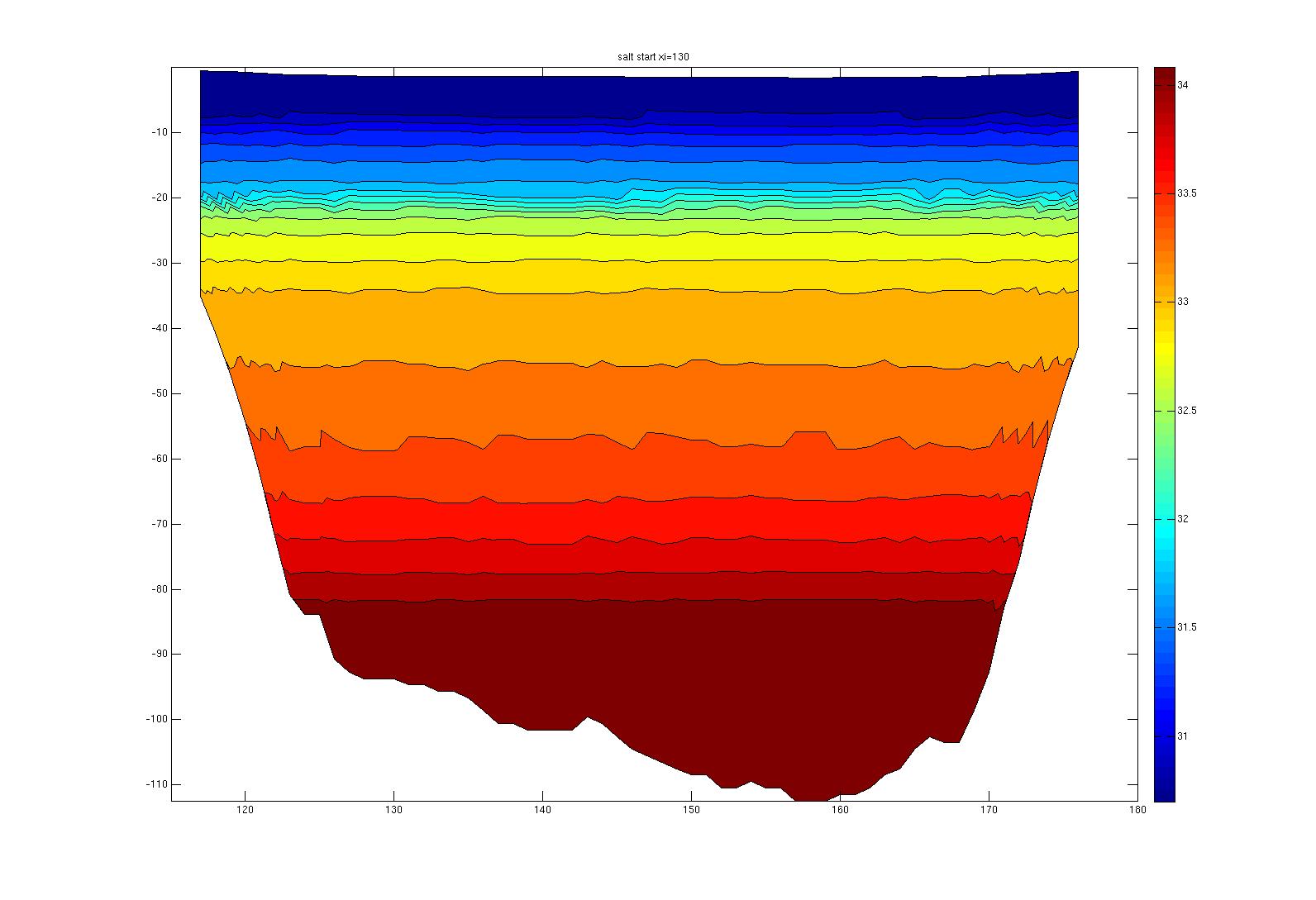
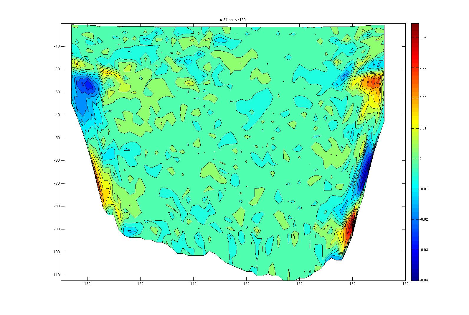
When checking my initialization file I realize that the I did not succeed in creating perfectly horizontal isolines. It may be that these errors induce the currents? Below are some images from the xi=130 crossection. From the first figure it is clear that the initial isolines are not horizontal everywhere. After 24 hours the salinity is smoothed out and apparently diffused somewhat downward in the lower layers, and tilted somewhat near the coast. The resulting pressure gradients differ in the vertical and induce the currents as shown.

https://www.myroms.org/links/t_1692/xi130_saltstart.jpg
https://www.myroms.org/links/t_1692/xi130_salt24.jpg
https://www.myroms.org/links/t_1692/xi130_u24.jpg

Below I attach the matlab used to generate the initial file.
Is there a better way to do this? What I have is a vector mysalt with salt values at set z-levels, constant salinity below 90m depth. Then I run though all the grid points, extract the z-values of each sigma layer in that point (using scoord.m from the utility package), and insert the correct salt value from the salt vector entry corresponding to the nearmost z-value. mk_vanm_init() is the main routine, and getSalt() is where the actual salt values are generated.

Eivind

Code: Select all

function [salt]=getSalt(zvec,mysalt)
% This function extracts salt values from mysalt, placing 
% them at sigmalayers given by zvec.
% Returns a vector of length ll=length(zvec)
%
% zvec: Vector of length ll, negative values where z(1) is the 
% deepmost value.
% mysalt: kk*2 matrix, first column gives salt values at negative z-values
% given in last column. mysalt(1,:) is the surface value

ll = length(zvec);
kk = length(mysalt(:,2));
salt = zeros(1,ll);
dz = abs(mysalt(1,2)-mysalt(2,2)); %Constant

for l=1:ll
    k=0;
    while (abs(zvec(l)-mysalt(kk-k,2))>=dz)
        k = k+1; 
    end
    if (k==kk || k==kk-1) %Surface
        salt(l) = mysalt(1,1);
    else
        dzz = abs(zvec(l)-mysalt(kk-k,2))/dz;
        salt(l) = dzz*mysalt(kk-k,1)+(1-dzz)*mysalt(kk-k+1,1); %Linear interpolation
    end
end

Code: Select all

function mk_vanm_init(mysalt)
fname = 'vanmini_hydro.nc';
h = nc_varget('vanm_grid.nc','h');

%Grid parametres, applies to Van Mijen only
dx = 200;
dy = 200;
Lx = dx*373;
Ly = dy*248;
xi_rho = 375 ;
xi_u = 374 ;
xi_v = 375 ;
eta_rho = 250 ;
eta_u = 250 ;
eta_v = 249 ;
s_rho = 32; % =N
s_w = 33; % = N+1

%Stretching parametres (must be similar to those in ocean_*.in):
Vtransf = 2;
Vstretch = 1;
theta_s = 1.0;
theta_b = 1.0;
Tcline = 25;

% Make x,y grid
xr = [-dx/2:dx:Lx+dx/2];
yr = [-dy/2:dy:Ly+dy/2]';
[xr,yr] = meshgrid(xr,yr);

% Get z, sigma and Cs-values
column = 0;
z_rho = zeros(eta_rho,xi_rho,s_rho);
z_w = zeros(eta_rho,xi_rho,s_w);
for index = 1:xi_rho
    [z_rho(:,index,:),sig_rho,Cs_r] = scoord(h, xr, yr, Vtransf, Vstretch,...
        theta_s, theta_b, Tcline, s_rho, 0, column, index, 0);
    [z_w(:,index,:),sig_w,Cs_w] = scoord(h, xr, yr, Vtransf, Vstretch,... 
        theta_s, theta_b, Tcline, s_rho, 1, column, index, 0);
end
sig_rho = sig_rho';
sig_w = sig_w';
Cs_r = Cs_r';
Cs_w = Cs_w';

%Temp data (constant = 2C everywhere):
temp = 2*ones(1,s_rho,eta_rho,xi_rho);

%Salt data:
% This setup: 
% I have a vector mysalt (257*2)
% mysalt(:,1): salinity values, constant below 90 m
% mysalt(:,2): z-value, dz=-0.625m
% 
% Need salt value at each s_rho, dependent on posistion. 
% z-values at each sigma layer l is given by
% z_rho(i,j,l)
% For each point i,j and layer l:
% - Go through mysalt, find where the z-value deviates by less than dz
% - Extract saltvalue


disp('Filling salt matrix..');
salt = zeros (1,s_rho,eta_rho,xi_rho);
landsalt = getSalt(squeeze(z_rho(1,1,:)),mysalt); % Standard vector over land
for j=1:xi_rho
    for i=1:eta_rho
        if h(i,j) == 3
            salt(1,:,i,j) = landsalt;
        else
            salt(1,:,i,j) = getSalt(squeeze(z_rho(i,j,:)),mysalt);
        end
    end
end


% Write to NetCDF file *************************
nc_varput ...
etc

mathieu
Posts: 74
Joined: Fri Sep 17, 2004 2:22 pm
Location: Institut Rudjer Boskovic

Re: Unphysical velocities using custom salinity

#5 Unread post by mathieu »

I believe you are a little too aggressive with the vertical parametrization. If you choose theta_s=4, theta_b=0.35, Vtransform=2, Vstrecthing=1 then the need for rx0 smoothing is much reduced.

In principle the higher theta_s the better the surface is resolved (at the expense of realism) and the lower your need of bathymetry smoothing. The higher theta_b the better the bottom is resolved and the higher the number N of vertical levels the higher the need for smoothing. But of course it is better to plot the levels before running the model.

eivinds
Posts: 8
Joined: Mon Sep 28, 2009 6:08 pm
Location: Geosciences, Univ. of Oslo

Re: Unphysical velocities using custom salinity

#6 Unread post by eivinds »

Thank you Mathieu for your reply.

I have changed the sigma layer parameters according to your suggestion. I also reduced the number of sigma layers from 32 to 24. I now smoothed first using GRID_LinProgHeuristic_rx0 with rmax=0.17, then applied GRID_Smooth_ROMS_rx1 with r1max=4.5. In addition I now use the ana_initial.h with a simplified analytical expression for the salinity distribution, to try remove errors in the matlab code. The code is attached below.

Even with the analytical salinity distribution and the rather smooth topography, ROMS is unable to represent the pycnocline in a horizontally homogenous way. See the attached figures. The first show a plot of the analytical function. The next is the initial density profile along the xi=130 section. The last is a snapshot of u-currents after 2 hours. What I find strange is that if I change the analytical function to a linear distribution on the form

Code: Select all

t(i,j,k,1,isalt)=30.7_r8-0.05_r8*z_r(i,j,k)
the resulting density distribution is near perfectly horizontally homogenous, and there are almost no currents generated at all.

Is there some connection between maximum Brunt Väisäälä frequency and topography / sigmalayer distribution that I have overlooked?

Eivind


Image
Image
Image

Code: Select all

# elif defined VANM
      DO k=1,N(ng)
        DO j=JstrR,JendR
          DO i=IstrR,IendR
            val1 = 29.813_r8+0.587_r8*EXP(-0.05_r8*z_r(i,j,k))
            val2 = 33.5_r8-1.7_r8*EXP(0.1_r8*(z_r(i,j,k)+20.0_r8))
            t(i,j,k,1,itemp)=2.0_r8
            depth = z_r(i,j,k)
            IF (depth.gt.-15.0_r8) THEN
              t(i,j,k,1,isalt)=val1
            ELSEIF (depth.lt.-25.0_r8) THEN
              t(i,j,k,1,isalt)=val2
            ELSE
              val3=(-depth-15.0_r8)/10.0_r8
              t(i,j,k,1,isalt)=(1.0_r8-val3*val3)*val1 + val3*val3*val2
            END IF
          END DO
        END DO
      END DO      

User avatar
kate
Posts: 4088
Joined: Wed Jul 02, 2003 5:29 pm
Location: CFOS/UAF, USA

Re: Unphysical velocities using custom salinity

#7 Unread post by kate »

There is a special case in the pressure gradient when the Brunt-Väisälä frequency is a constant - the errors drop out.

I tried to use lpsolve to come up with a steeper working bathymetry form Northeast Pacific grid and failed. I'm back to using the very smooth bathymetry from before because the model likes it better.

Post Reply